
Section 4.4 kinematic analysis of simple rigid body systems

Subsection 4.4.1 simply supported beam

Perform the kinematic analysis of the following beam of length equal to \(l\text{.}\)

Figure 4.4.1.

By “reading” the applyed constraints the following equations can be written

\begin{gather*} \vec{u}_A = \vec0\,,\\ \vec{u}_B \cdot \vec{n}_B = 0\,, \end{gather*}

where \(\vec{n}_B = \transp{[0 \; 1]}\text{.}\) Previous equations can be also expressed by the following 3 scalar equations (\(m=3\)):

\begin{gather*} u_{1A} = 0\,,\\ u_{2A} = 0\,,\\ u_{2B} = 0\,. \end{gather*}

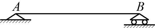
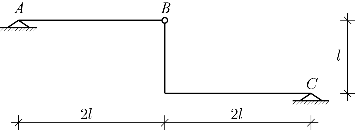
For the only rigid body in question, choose point \(A \) as the pole, therefore the 3 Lagrangian parameters (\(n = 3 \)) that can be used for the kinematic description of the system are:

Figure 4.4.2.
Using the equation (4.1.5) the constraint conditions can be expressed with respect to the chosen Lagrangian coordinates

\begin{gather*} u_{1A} = 0\,,\\ u_{2A} = 0\,,\\ u_{2A} + \varphi_{A} l = 0\,. \end{gather*}

Conditions which give

\begin{equation*} \underbrace{\left[\begin{array}{ccc} 1 & 0 & 0\\ 0 & 1 & 0\\ 0 & 1 & l \end{array}\right]}_{\mat{A}} \underbrace{\left[\begin{array}{c} u_{1A} \\ u_{2A} \\ \varphi_{A} \end{array}\right]}_{\vec{q}} = \underbrace{\left[\begin{array}{c} 0 \\ 0 \\ 0 \end{array}\right]}_{\vec{d}}. \end{equation*}

Before proceeding with the solution of the system, it is possible to classify the system by calculating the rank of the kinematic matrix using the following MATLAB® instructions.

syms l;
A = [1 0 0; 0 1 0; 0 1 l];
rank(A)
Listing 4.4.3.

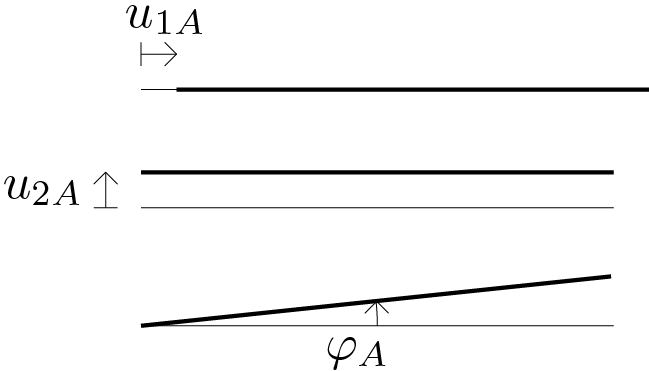
Since the \(\textrm{min} (m, n) = 3 == \text{rank} \ mat {A} \) and \(n == m \) then the system is kinematically determined. Finally, the solution of the linear system provides the values assumed by the Lagrangian parameters \(u_{1A} \text{,}\) \(u_{2A} \) and \(\varphi_{A} \) which, in this case, are identically null.

syms l;
A = [1 0 0; 0 1 0; 0 1 l];
b = [0; 0; 0];
linsolve(A,b)
Listing 4.4.4.

Let us assume to modify the assigned system as follows.

Figure 4.4.5.
In this case it is necessary to simply modify the constraint condition for the roller support placed in point \(B \text{,}\) that is

\begin{equation*} u_{2B} = l/10\,. \end{equation*}

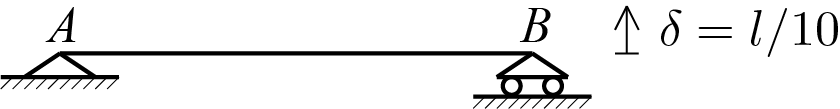
Therefore on the system of equations to be analyzed, the only effect is constituted by the modification of the vector of the known terms and there is no effect on the classification of the system which always remains kinematically determined (the matrix \(A \) has not changed). Therefore the system of equations becomes

\begin{equation*} \underbrace{\left[\begin{array}{ccc} 1 & 0 & 0\\ 0 & 1 & 0\\ 0 & 1 & l \end{array}\right]}_{\mat{A}} \underbrace{\left[\begin{array}{c} u_{1A} \\ u_{2A} \\ \varphi_{A} \end{array}\right]}_{\vec{q}} = \underbrace{\left[\begin{array}{c} 0 \\ 0 \\ l/10 \end{array}\right]}_{\vec{d}}. \end{equation*}

The solution of the linear system provides the new values assumed by the Lagrangian parameters \(u_{1A} \text{,}\) \(u_{2A} \) and \(\varphi_{A} \text{.}\)

syms l;
A = [1 0 0; 0 1 0; 0 1 l];
b = [0; 0; l/10];
linsolve(A,b)
Listing 4.4.6.

Subsection 4.4.2 L shaped beam with 3 roller supports

The assigned system is shown in the figure below.

Figure 4.4.7.

The proposed scheme does not present any particular novelty with respect to the previous scheme and the following MATLAB® instructions allow to obtain the desired solution.

% generic 2D displacement for a rigid body
rigidDispl = ...
    @(u0, phi0, X0, X)...
    [u0(1)-phi0*(X(2)-X0(2));...
     u0(2)+phi0*(X(1)-X0(1))];

% geometric description of the beam
syms l;
A = [0; 0];
B = [l; 0];
C = [l; l/2];

% displacement description by using the point A as pole
POLE = A;
syms phiA;
phi0 = phiA;
u0 = sym('uA', [2 1]);
uA = rigidDispl(u0, phi0, POLE, A);
uB = rigidDispl(u0, phi0, POLE, B);
uC = rigidDispl(u0, phi0, POLE, C);

% constraint equations
eqns = [
uA(2) == 0,
uB(2) == 0,
uC(1) == 0
];

% kinematic matrix and vector of the assigned displacements
[A,d] = equationsToMatrix(eqns, [uA(1), uA(2), phiA]);

% degrees of freedom, n
% number of constrains, m
[m,n] = size(A); 

% rank of A
r = rank(A);

% if the system is kinematically determined the solution is calculated
if and(r == min(m,n), m == n)
    x = linsolve(A,d);
end
Listing 4.4.8.

Subsection 4.4.3 system with three hinges

Perform the kinematic analysis of the following system.

Figure 4.4.9.

The “reading” of the assigned constraint conditions gives

\begin{gather*} \vec{u}_A = \vec{0}\,,\\ \vec{u}_B = \vec{u}_{B'}\,,\\ \vec{u}_C = \vec0\,, \end{gather*}

which can be also expressed by the following scalar equations (\(m=6\)):

\begin{gather*} u_{1A} = 0\,,\\ u_{2A} = 0\,,\\ u_{1B} = u_{1B'}\,,\\ u_{2B} = u_{2B'}\,,\\ u_{1C} = 0\,,\\ u_{2C} = 0\,. \end{gather*}

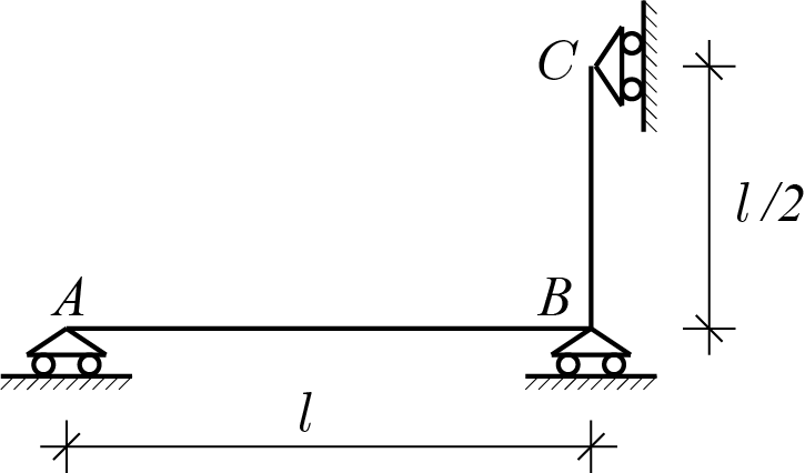
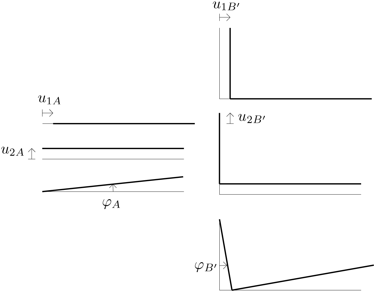
The rigid bodies under examination are two: for the body \(AB \) the point \(A \) is chosen as the pole and for the second body the point \(B'\) is chosen. Therefore the 6 Lagrangian parameters (\(n = 6 \)) adopted for the kinematic description of the system are:

Figure 4.4.10.
Using the equation (4.1.5) the constraint conditions can be expressed with respect to the chosen Lagrangian coordinates, in particular:

\begin{gather*} u_{1A} = 0\,,\\ u_{2A} = 0\,,\\ u_{1A} = u_{1B'}\,,\\ u_{2A} + \varphi_{A} 2l = u_{2B'}\,,\\ u_{1B'} + \varphi_{B'} l = 0\,,\\ u_{2B'} + \varphi_{B'} 2l = 0\,. \end{gather*}

or, in matrix format,

\begin{equation*} \underbrace{\left[\begin{array}{cccccc} 1 & 0 & 0 & 0 & 0 & 0\\ 0 & 1 & 0 & 0 & 0 & 0\\ 1 & 0 & 0 & -1 & 0 & 0\\ 0 & 1 & 2l & 0 & -1 & 0\\ 0 & 0 & 0 & 1 & 0 & l\\ 0 & 0 & 0 & 0 & 1 & 2l \end{array}\right]}_{\mat{A}} \underbrace{\left[\begin{array}{c} u_{1A} \\ u_{2A} \\ \varphi_{A} \\ u_{1B'} \\ u_{2B'} \\ \varphi_{B'} \end{array}\right]}_{\vec{q}} = \underbrace{\left[\begin{array}{c} 0 \\ 0 \\ 0 \\ 0 \\ 0 \\ 0 \end{array}\right]}_{\vec{d}}. \end{equation*}

In order to classify the system, the rank of the kinematic matrix is calculated.

syms l;
A = [
1 0 0 0 0 0; ... 
0 1 0 0 0 0; ... 
1 0 0 -1 0 0; ...
0 1 2*l 0 -1 0; ...
0 0 0 1 0 l; ...
0 0 0 0 1 2*l ...
];
rank(A)
Listing 4.4.11.

Since \(\textrm{min}(m,n) = 6 == \textrm{rango}\mat{A}\) and \(n == m\) then the system is kinematically determined. The solution of the linear system provides the values assumed by the Lagrangian parameters \(u_{1A}\text{,}\) \(u_{2A}\text{,}\) \(\varphi_{A}\text{,}\) \(u_{1B'}\text{,}\) \(u_{2B'}\text{,}\) \(\varphi_{B'}\text{.}\)

syms l;
A = [
1 0 0 0 0 0; ... 
0 1 0 0 0 0; ... 
1 0 0 -1 0 0; ...
0 1 2*l 0 -1 0; ...
0 0 0 1 0 l; ...
0 0 0 0 1 2*l ...
];
b = [0; 0; 0; 0; 0; 0];
linsolve(A,b)
Listing 4.4.12.

Also in this case the solution of a kinematically determined system with respect to a vector of the known terms which is identically null still provides the trivial solution.

A more interesting result can be obtained by assuming an assigned non-zero displacement condition on one or more degrees of constraint. For example:

Figure 4.4.13.
In this case the matrix form of the constraint conditions provides

\begin{equation*} \underbrace{\left[\begin{array}{cccccc} 1 & 0 & 0 & 0 & 0 & 0\\ 0 & 1 & 0 & 0 & 0 & 0\\ 1 & 0 & 0 & -1 & 0 & 0\\ 0 & 1 & 2l & 0 & -1 & 0\\ 0 & 0 & 0 & 1 & 0 & l\\ 0 & 0 & 0 & 0 & 1 & 2l \end{array}\right]}_{\mat{A}} \underbrace{\left[\begin{array}{c} u_{1A} \\ u_{2A} \\ \varphi_{A} \\ u_{1B'} \\ u_{2B'} \\ \varphi_{B'} \end{array}\right]}_{\vec{q}} = \underbrace{\left[\begin{array}{c} l/4 \\ 0 \\ 0 \\ 0 \\ 0 \\ 0 \end{array}\right]}_{\vec{d}}\,. \end{equation*}

The solution can be calculated using the following MATLAB® instructions.

syms l;
A = [
1 0 0 0 0 0; ... 
0 1 0 0 0 0; ... 
1 0 0 -1 0 0; ...
0 1 2*l 0 -1 0; ...
0 0 0 1 0 l; ...
0 0 0 0 1 2*l ...
];
b = [l/4; 0; 0; 0; 0; 0];
linsolve(A,b)
Listing 4.4.14.

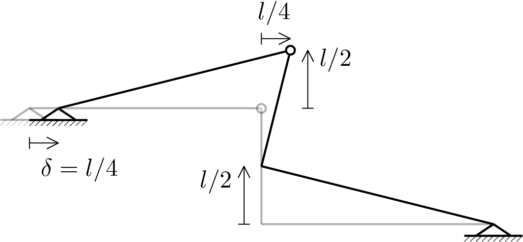
The graphical representation of the displacement field is obtained by evaluating the displacement of the end points of the straight parts of the beams, obtaining what follows.

Figure 4.4.15.

The following MATLAB® instructions allow you to obtain a plot of the kinematics shown above.

% geometric description
L = 100;
A = [0; 0];
B = [2*L; 0];
C = [2*L; -L];
D = [4*L; -L];
beam1 = [A B];
beam2 = [B C D];

% function for the evaluation of the new position of a point
rigidT = @(u0, X0, phi0, X) ...
[X(1)+u0(1)-phi0*(X(2)-X0(2)); ...
X(2)+u0(2)+phi0*(X(1)-X0(1))];

% new configuration of the first beam (pole in A)
u0 = [L/4; 0];
phi0 = 1/4;
X0 = A;
TA = rigidT(u0, X0, phi0, A);
TB = rigidT(u0, X0, phi0, B);
beam1T = [TA TB];

% new configuration of the first beam (pole in D)
u0 = [0; 0];
phi0 = -1/4;
X0 = D;
TC = rigidT(u0, X0, phi0, C);
TD = rigidT(u0, X0, phi0, D);
beam2T = [TB TC TD];

% drawing
clf

x = beam1(1,:);
y = beam1(2,:);
line(x,y,'LineWidth',2,'Color','black')

x = beam2(1,:);
y = beam2(2,:);
line(x,y,'LineWidth',2,'Color','black')

x = beam1T(1,:);
y = beam1T(2,:);
line(x,y,'LineWidth',2,'Color','red')

x = beam2T(1,:);
y = beam2T(2,:);
line(x,y,'LineWidth',2,'Color','red')

xlim([0 4*L])
ylim([-L 0.5*L])
pbaspect([2.667 1 1])
Listing 4.4.16.

Subsection 4.4.4 mechanism example

Perform the kinematic analysis of the following system.

Figure 4.4.17.

The constraint conditions assigned can be expressed as follows

\begin{gather*} \vec{u}_A = \vec{0}\,,\\ \vec{u}_C = \vec{u}_{C'}\,, \end{gather*}

The corresponding set of scalar equations is (\(m=5\)):

\begin{gather*} u_{1A} = 0\,,\\ u_{2A} = 0\,,\\ u_{1C} = u_{1C'}\,,\\ u_{2C} = u_{2C'}\,,\\ u_{2E} = 0\,. \end{gather*}

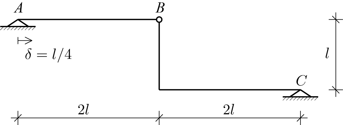
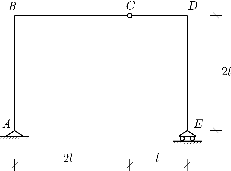
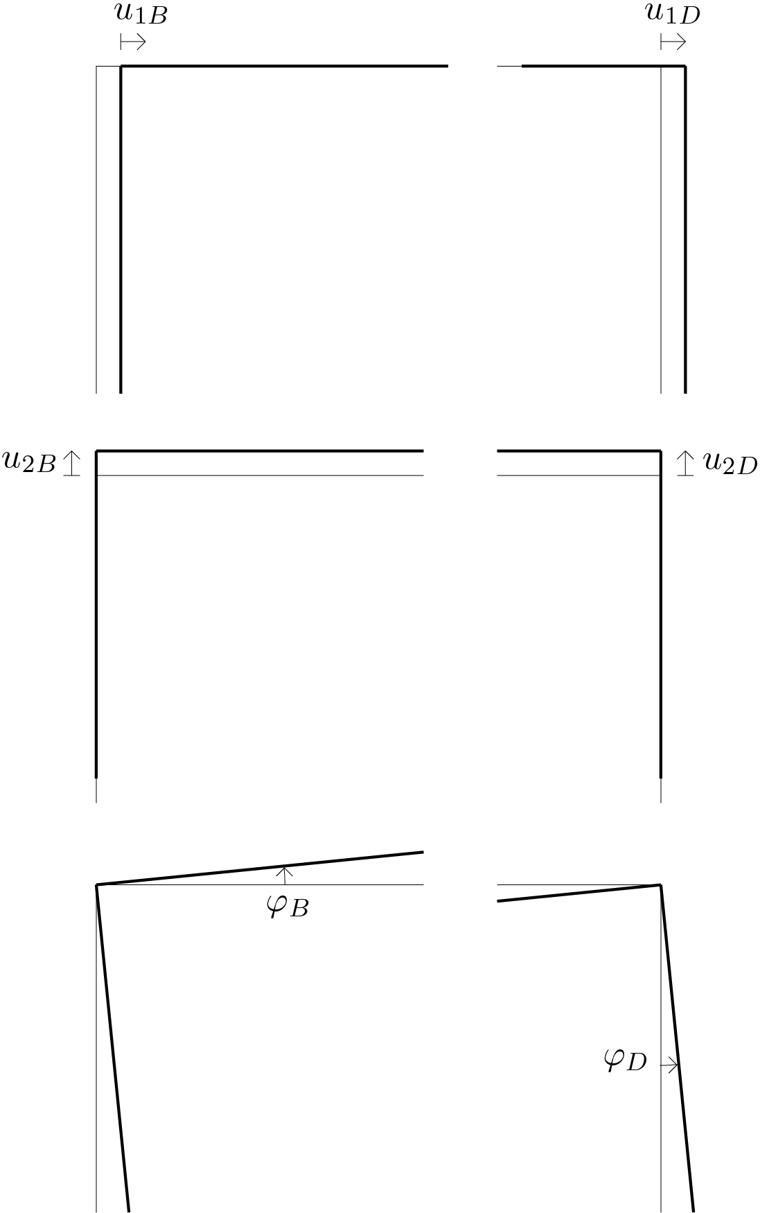
For the two rigid bodies under examination, points B and D are chosen as poles, thus the kinematics is described through the following 6 Lagrangian parameters (\(n=6\)):

Figure 4.4.18.
Always using the plane motion model represented by the equation (4.1.5) the constraint conditions can be expressed with respect to the chosen Lagrangian coordinates obtaining the following result,

\begin{gather*} u_{1B} + \varphi_{B} 2l = 0\,,\\ u_{2B} = 0\,,\\ u_{1B} = u_{1D}\,,\\ u_{2B} + \varphi_{B} 2l = u_{2D}-\varphi_{D} l\,,\\ u_{2D} = 0\,. \end{gather*}

Using a matrix format, the system of constraint equations can be written as

\begin{equation*} \underbrace{\left[\begin{array}{cccccc} 1 & 0 & 2l & 0 & 0 & 0\\ 0 & 1 & 0 & 0 & 0 & 0\\ 1 & 0 & 0 & -1 & 0 & 0\\ 0 & 1 & 2l & 0 & -1 & l\\ 0 & 0 & 0 & 0 & 1 & 0 \end{array}\right]}_{\mat{A}} \underbrace{\left[\begin{array}{c} u_{1B} \\ u_{2B} \\ \varphi_{B} \\ u_{1D} \\ u_{2D} \\ \varphi_{D} \end{array}\right]}_{\vec{q}} = \underbrace{\left[\begin{array}{c} 0 \\ 0 \\ 0 \\ 0 \\ 0 \end{array}\right]}_{\vec{d}}. \end{equation*}

It is possible to proceed with the calculation of the rank of the matrix as follows.

syms l;
A = [
1 0 2*l 0 0 0; ... 
0 1 0 0 0 0; ... 
1 0 0 -1 0 0; ...
0 1 2*l 0 -1 l; ...
0 0 0 0 1 0; ...
];
rank(A)
Listing 4.4.19.

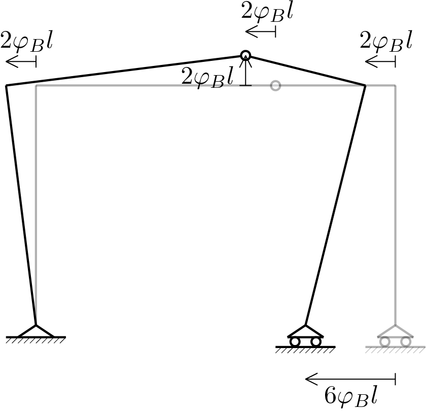
In the present case \(\textrm{rango}\mat{A} == \textrm{min}(m,n) = 5\) and \(m < n\) therefore the system is a mechanism and characterized by infinite solutions. To describe all possible solutions, choose the rotation \(\varphi_{B}\) as parameter to be eliminated from the group of unknowns. In this way the system can be rewritten as follows

\begin{equation*} \left[\begin{array}{ccccc} 1 & 0 & 0 & 0 & 0\\ 0 & 1 & 0 & 0 & 0\\ 1 & 0 & -1 & 0 & 0\\ 0 & 1 & 0 & -1 & l\\ 0 & 0 & 0 & 1 & 0 \end{array}\right] \left[\begin{array}{c} u_{1B} \\ u_{2B} \\ u_{1D} \\ u_{2D} \\ \varphi_{D} \end{array}\right] = \left[\begin{array}{c} -2l\,\varphi_{B} \\ 0 \\ 0 \\ -2l\,\varphi_{B} \\ 0 \end{array}\right]. \end{equation*}

The following MATLAB® instructions allow to calculate the solution we are looking for.

syms l k;
A = [
1 0 0 0 0; ... 
0 1 0 0 0; ... 
1 0 -1 0 0; ...
0 1 0 -1 l; ...
0 0 0 1 0; ...
];
b = [-2*l*k; 0; 0; -2*l*k; 0];
linsolve(A,b)
Listing 4.4.20.

The obtained infinite solutions are

\begin{gather*} u_{1B} = -\varphi_{B} 2l \,,\\ u_{2B} = 0\,,\\ u_{1D} = -\varphi_{B} 2l\,,\\ u_{2D} = 0\,,\\ \varphi_{D} = - 2\varphi_{B} \,. \end{gather*}

One of these can be represented as follows

Figure 4.4.21.

Subsection 4.4.5 esercizi proposti

Perform the previous exercises by suitably modifying the MATLAB® code used for the example shown in Subsection 4.4.2.