
Section 3.3 multi-axial states

Subsection 3.3.1 the model as a generalization of Hooke's law

The uniaxial states of traction/compression and shear highlighted two different experimental parameters, the Young \(E \) modulus and the shear modulus \(G \text{,}\) usable as proportionality coefficients in the definition of the elastic relationship existing between the stress component and its strain component. In order to extend this approach to multi-axial states, the definition of elastic relationships has to be capable to describe more complex situations in which the stress components, in general, do not depend only on the corresponding strain components. Therefore the following proportionality coefficients are introduced

Figure 3.3.1.
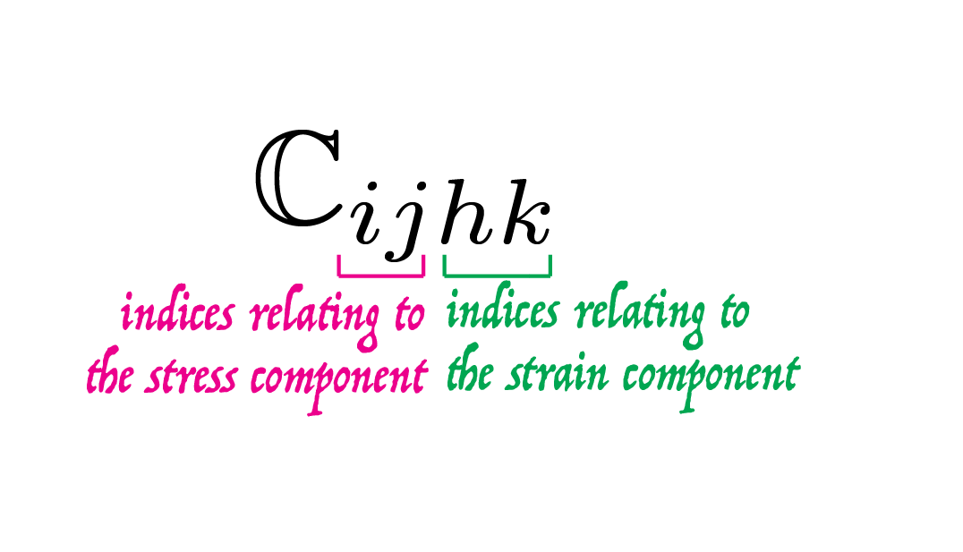
between the generic stress component \(\sigma_{ij} \) and the generic strain component \(\varepsilon_ {hk} \text{.}\) So for each of the 9 stress components (\(i, \, j = 1 \dots 3 \)) it will be necessary to define as many coefficients of proportionality as the strain components, which are also 9 (\(h, \, k = 1 \dots 3 \)). Each contribution given by the generic strain component can be added together by providing

\begin{align*} \sigma_{ij} \amp = \mathbb{C}_{ij11}\,\varepsilon_{11} + \mathbb{C}_{ij12}\,\varepsilon_{12} + \mathbb{C}_{ij13}\,\varepsilon_{13} \,+ \\ \amp + \mathbb{C}_{ij21}\,\varepsilon_{21} + \mathbb{C}_{ij22}\,\varepsilon_{22} + \mathbb{C}_{ij23}\,\varepsilon_{23} \,+ \\ \amp + \mathbb{C}_{ij31}\,\varepsilon_{31} + \mathbb{C}_{ij32}\,\varepsilon_{32} + \mathbb{C}_{ij33}\,\varepsilon_{33}\,. \end{align*}

There are therefore 9 proportionality coefficients for each of the 9 stress components for a total of 81 coefficients. This relationship can be expressed in compact form as like

\begin{equation} \sigma_{ij} = \sum_{h,k=1 \dots 3}\mathbb{C}_{ijhk}\varepsilon_{hk} \label{components_costitutivo_continuo_eq}\tag{3.3.1} \end{equation}

or, in tensorial form, by writing

\begin{equation} \tens{\sigma} = \tensQ{C}:\tens{\varepsilon} \label{costitutivo_continuo_eq}\tag{3.3.2} \end{equation}

relationship that highlights a new type of linear transformation that associates the generic strain tensor with the corresponding stress tensor. In this case, the linear operator involved is given by the 4th order tensor \(\tensQ{C} \text{,}\) the tensor which internally contains the above 81 coefficients.

It is also assumed the possibility of defining elastic energy for multi-axial states as follows

\begin{equation} \Phi = \frac{1}{2} \tens{\sigma}:\tens{\varepsilon}\,,\tag{3.3.3} \end{equation}

quantity which, as for the uniaxial case, represents half of the internal work, that is the work carried out by the stress on the strain. Elastic energy, on the basis of the constitutive relationship (3.3.2), can be rewritten as follows

\begin{equation} \Phi = \frac{1}{2} \left( \tensQ{C}:\tens{\varepsilon} \right):\tens{\varepsilon}\,.\label{energia_continuo_eq}\tag{3.3.4} \end{equation}

Subsubsection 3.3.1.1 properties of the constitutive tensor

  • The definition of energy, Eq. (3.3.4), and the condition of non-negativity of internal work imply that the constitutive tensor must necessarily be defined positive, that is
    \begin{equation*} \left(\tensQ{C}:\tens{\varepsilon}\right):\tens{\varepsilon} \geq 0 \end{equation*}
    and the only case which is null occurs when \(\tens{\varepsilon} = \tens{0} \text{.}\)
  • By definition of elastic potential, the relationship between generic stress component \(\sigma_{ij} \) and elastic energy can be written as
    \begin{equation} \sigma_{ij} = \frac{\partial \Phi}{\partial \varepsilon_{ij}}\,.\tag{3.3.5} \end{equation}
    Further deriving this relationship and using relationship (3.3.1) we obtain
    \begin{equation*} \frac{\partial}{\partial \varepsilon_{hk}} \left(\frac{\partial \Phi}{\partial \varepsilon_{ij}}\right) = \frac{\partial}{\partial \varepsilon_{hk}} \left(\sigma_{ij}\right) = \frac{\partial}{\partial \varepsilon_{hk}} \left(\sum_{h,k=1 \dots 3}\mathbb{C}_{ijhk}\varepsilon_{hk} \right) = \mathbb{C}_{ijhk} \,. \end{equation*}
    Therefore the generic coefficient of the constitutive tensor is related to the elastic energy through relationship
    \begin{equation} \mathbb{C}_{ijhk} = \frac{\partial}{\partial \varepsilon_{hk}} \left(\frac{\partial \Phi}{\partial \varepsilon_{ij}}\right)\,.\tag{3.3.6} \end{equation}
    Observing that by swapping the derivation order the result does not change
    \begin{equation*} \mathbb{C}_{ijhk} = \frac{\partial}{\partial \varepsilon_{hk}} \left(\frac{\partial \Phi}{\partial \varepsilon_{ij}}\right) = \frac{\partial}{\partial \varepsilon_{ij}} \left(\frac{\partial \Phi}{\partial \varepsilon_{hk}}\right) = \frac{\partial}{\partial \varepsilon_{ij}} \left(\sigma_{hk} \right) = \mathbb{C}_{hkij}\,, \end{equation*}
    followin condition is fulfilled
    \begin{equation} \mathbb{C}_{ijhk} = \mathbb{C}_{hkij}\tag{3.3.7} \end{equation}
    known as major symmetry of the constitutive tensor \(\tensQ{C} \text{.}\)
  • The symmetry of the stress components allows to write
    \begin{equation} \mathbb{C}_{ijhk} = \mathbb{C}_{jihk}\,,\tag{3.3.8} \end{equation}
    while the symmetry condition of the strain components provides
    \begin{equation} \mathbb{C}_{ijhk} = \mathbb{C}_{ijkh}\,.\tag{3.3.9} \end{equation}
    These conditions are called minor symmetries of the tensor \(\tensQ{C} \text{.}\)
  • The symmetry conditions described above reduce the number of effectively independent coefficients necessary to define a generic elastic tensor from 81 to 21.

Subsection 3.3.2 experimental observation

The main phenomenon highlighted by the experimental observation of multiaxial stress / strain states is that the application of a load in an assigned direction determines not only a deformation along that direction but also along the directions transverse to it. This phenomenon, as shown also in the following animation, is observed in particular for the states of traction or compression and is called Poisson effect.

For simpler materials Poisson effect is modeled through the introduction of a single characteristic parameter of the material, known as the Poisson coefficient, which links the generic transverse strain to the strain relative to the direction of the applied load. For example, if a stress \(\sigma_{11} \) is applied, the strain along the direction of the load will take on a generic value

\begin{equation*} \varepsilon_{11}\,, \end{equation*}

while the strains in the transverse directions will be

\begin{equation*} \varepsilon_{22} = -\nu\,\varepsilon_{11}\,,\qquad \varepsilon_{33} = -\nu\,\varepsilon_{11}\,, \end{equation*}

where \(\nu\) is precisely the Poisson coefficient.

Subsection 3.3.3 the isotropic case

The experimental parameters encountered so far are Young's modulus, \(E \text{,}\) the shear modulus, \(G \) and the Poisson's ratio, \(\ nu \) . It has also been said, see previous section, that the number of coefficients strictly necessary to define the constitutive tensor is equal to 21. It therefore seems that the experimental results discussed so far are very insufficient to reach a complete definition of the elastic relationship. Fortunately, most of the materials used in the usual engineering applications are isotropic. That is, they have the property that, given a block of material and any direction is chosen to cross it by means of experimental tests, the same mechanical response is always detected. For this class of materials, applicable to metals, glass, polymers, soils and, in some ways, even cement or bituminous conglomerates, the constitutive characterization can be carried out by only 2 experimental parameters.

A couple of experimental parameters, although not the only pair, is given by the pair formed by Young's modulus parameters, \(E \) and Poisson's ratio, \(\nu \text{.}\) The shear modulus \(G \) depends in fact on \(E \) and \(\nu \) according to the following formula

\begin{equation} G = \frac{E}{2\left(1+\nu\right)}\,.\tag{3.3.10} \end{equation}

Given this, it is convenient to discuss the elastic and isotropic material behavior by keeping the strain/stress components of the normal type and the tangential type components separate since, for isotropic materials, there is no coupling and therefore the coefficients of the type

\begin{equation*} \mathbb{C}_{iihk}\;\text{con}\; h \neq k \end{equation*}

are however null.

Subsubsection 3.3.3.1 normal components

The elastic relationship for normal components can be formulated as follows

\begin{equation} \begin{array}{rcrcrcr} \varepsilon_{11} = \amp + \amp \frac{\displaystyle\sigma_{11}}{\displaystyle E} \amp-\amp \nu\,\frac{\displaystyle\sigma_{22}}{\displaystyle E} \amp-\amp \nu\,\frac{\displaystyle \sigma_{33}}{\displaystyle E}\,,\\ \varepsilon_{22} = \amp - \amp \nu\,\frac{\displaystyle \sigma_{11}}{\displaystyle E} \amp+\amp \frac{\displaystyle \sigma_{22}}{\displaystyle E} \amp-\amp \nu\,\frac{\displaystyle \sigma_{33}}{\displaystyle E}\,,\\ \varepsilon_{33} = \amp - \amp \nu\,\frac{\displaystyle \sigma_{11}}{\displaystyle E} \amp-\amp \nu\,\frac{\displaystyle \sigma_{22}}{\displaystyle E} \amp+\amp \frac{\displaystyle \sigma_{33}}{\displaystyle E}\,. \end{array}\label{isotropic_normal_eq}\tag{3.3.11} \end{equation}

It is observed that this result constitutes the inverse form of the elastic relationship for the part relating to the normal components. To obtain the elastic coefficients that proportionally correlate the stress components to the strain components, it is better to visualize the relationship in the following matrix form

\begin{equation*} \left[\begin{array}{c}\varepsilon_{11} \\ \varepsilon_{22} \\ \varepsilon_{33}\end{array}\right] = \left[\begin{array}{ccc} \frac{\displaystyle 1}{\displaystyle E} \amp -\frac{\displaystyle \nu}{\displaystyle E} \amp -\frac{\displaystyle \nu}{\displaystyle E} \\ -\frac{\displaystyle \nu}{\displaystyle E} \amp \frac{\displaystyle 1}{\displaystyle E} \amp -\frac{\displaystyle \nu}{\displaystyle E} \\ -\frac{\displaystyle \nu}{\displaystyle E} \amp -\frac{\displaystyle \nu}{\displaystyle E} \amp \frac{\displaystyle 1}{\displaystyle E} \\ \end{array}\right] \left[\begin{array}{c}\sigma_{11} \\ \sigma_{22} \\ \sigma_{33}\end{array}\right] \end{equation*}

and use the following MATLAB® instructions to invert the highlighted matrix.

syms E ni;
M = [1/E -ni/E -ni/E; -ni/E 1/E  -ni/E; -ni/E -ni/E 1/E]
inv(M)
Listing 3.3.2.
So we get

\begin{equation} \left[\begin{array}{c}\sigma_{11} \\ \sigma_{22} \\ \sigma_{33}\end{array}\right] = \frac{E}{(1+\nu)(1-2\nu)} \left[\begin{array}{ccc} (1-\nu) \amp \nu \amp \nu \\ \nu \amp (1-\nu) \amp \nu \\ \nu \amp \nu \amp (1-\nu) \end{array}\right] \left[\begin{array}{c}\varepsilon_{11} \\ \varepsilon_{22} \\ \varepsilon_{33}\end{array}\right]\,.\tag{3.3.12} \end{equation}

Result that allows to identify the non-zero constitutive coefficients relative to the normal components of the stress tensor, that is

\begin{gather} \mathbb{C}_{1111} = \mathbb{C}_{2222} = \mathbb{C}_{3333} = \frac{E(1-\nu)}{(1+\nu)(1-2\nu)}\,,\tag{3.3.13}\\ \mathbb{C}_{1122} = \mathbb{C}_{1133} = \mathbb{C}_{2233} = \frac{E\,\nu}{(1+\nu)(1-2\nu)}\,,\tag{3.3.14}\\ \mathbb{C}_{2211} = \mathbb{C}_{1122}\,,\tag{3.3.15}\\ \mathbb{C}_{3311} = \mathbb{C}_{1133}\,,\tag{3.3.16}\\ \mathbb{C}_{3322} = \mathbb{C}_{2233}\,.\tag{3.3.17} \end{gather}

Subsubsection 3.3.3.2 tangential type components

For tangential components, in addition to the absence of coupling with normal components, it is not necessary to model any reciprocal coupling, therefore for all tangential components the uniaxial law already seen in Subsection 3.2.2 can be assumed

\begin{equation} \begin{array}{rr} \gamma_{23} = 2\,\varepsilon_{23} = \amp \frac{\displaystyle \sigma_{23}}{\displaystyle G}\,,\\ \gamma_{31} = 2\,\varepsilon_{31} = \amp \frac{\displaystyle \sigma_{31}}{\displaystyle G}\,,\\ \gamma_{12} = 2\,\varepsilon_{12} = \amp \frac{\displaystyle \sigma_{12}}{\displaystyle G}\,. \end{array}\tag{3.3.18} \end{equation}
From which the following relationship is obtained between the tangential components of the stress and strain tensors
\begin{equation} \sigma_{23} = 2\,G\,\varepsilon_{23}\,,\quad \sigma_{31} = 2\,G\,\varepsilon_{31}\,,\quad \sigma_{12} = 2\,G\,\varepsilon_{12}\,,\tag{3.3.19} \end{equation}
and therefore the following non-zero constitutive coefficients
\begin{equation} \mathbb{C}_{2323} = \mathbb{C}_{3131} = \mathbb{C}_{1212} = 2\,G\,.\tag{3.3.20} \end{equation}

Subsubsection 3.3.3.3 summary and Voigt notation

In the previous discussion, the elastic law was presented keeping the description of the part concerning the normal components separate from that relating to the tangential components. This certainly to better highlight the lack of certain couplings between stress components and strain components, but also for the impossibility of representing in a compact way the components of a 4th tensor such as the constitutive tensor. In fact, while for the tensors of the 2nd order the representation of all the components is realized through the associated matrix, for a 4th tensor there is no similar representation.

A summary of what described above can be obtained using the Voigt notation which uses 6-component vectors to represent 2nd order symmetric tensors, while for the corresponding 4th order tensors 1  6\(\times\)6 matrices. Therefore the constitutive elastic law can be written as follows

\begin{equation} \left[\begin{array}{c}\sigma_{11} \\ \sigma_{22} \\ \sigma_{33} \\ \sigma_{23} \\ \sigma_{31} \\ \sigma_{12}\end{array}\right] = \frac{E}{(1+\nu)(1-2\nu)} \left[\begin{array}{cccccc} (1-\nu) \amp \nu \amp \nu \amp 0 \amp 0 \amp 0\\ \nu \amp (1-\nu) \amp \nu \amp 0 \amp 0 \amp 0\\ \nu \amp \nu \amp (1-\nu) \amp 0 \amp 0 \amp 0\\ 0 \amp 0 \amp 0 \amp (1-2\nu)/2 \amp 0 \amp 0 \\ 0 \amp 0 \amp 0 \amp 0 \amp (1-2\nu)/2 \amp 0 \\ 0 \amp 0 \amp 0 \amp 0 \amp 0 \amp (1-2\nu)/2 \end{array}\right] \left[\begin{array}{c}\varepsilon_{11} \\ \varepsilon_{22} \\ \varepsilon_{33} \\ 2\,\varepsilon_{23} \\ 2\,\varepsilon_{31} \\ 2\,\varepsilon_{12}\end{array}\right]\,.\tag{3.3.21} \end{equation}
Corresponding in the sense of 4th order tensors which map 2nd symmetric tensors into 2nd order symmetric tensors.

For completeness, a summary of the elastic and isotropic law is also provided using the tensor format.

\begin{equation} \tens{\sigma} = \tensQ{C}:\tens{\varepsilon} \tag{3.3.22} \end{equation}

where the non-zero components of tensor \(\tensQ{C}\) are

\begin{align} \amp\mathbb{C}_{1111} = \mathbb{C}_{2222} = \mathbb{C}_{3333} = \frac{E(1-\nu)}{(1+\nu)(1-2\nu)}\,,\tag{3.3.23}\\ \amp\mathbb{C}_{1122} = \mathbb{C}_{1133} = \mathbb{C}_{2233} =\tag{3.3.24}\\ \amp\mathbb{C}_{2211} = \mathbb{C}_{3311} = \mathbb{C}_{3322} = \frac{E\,\nu}{(1+\nu)(1-2\nu)}\,,\tag{3.3.25}\\ \amp\mathbb{C}_{2323} = \mathbb{C}_{3131} = \mathbb{C}_{1212} = 2\,G\,.\tag{3.3.26} \end{align}