A first course on solid mechanics

Section 1.3 deformation gradient

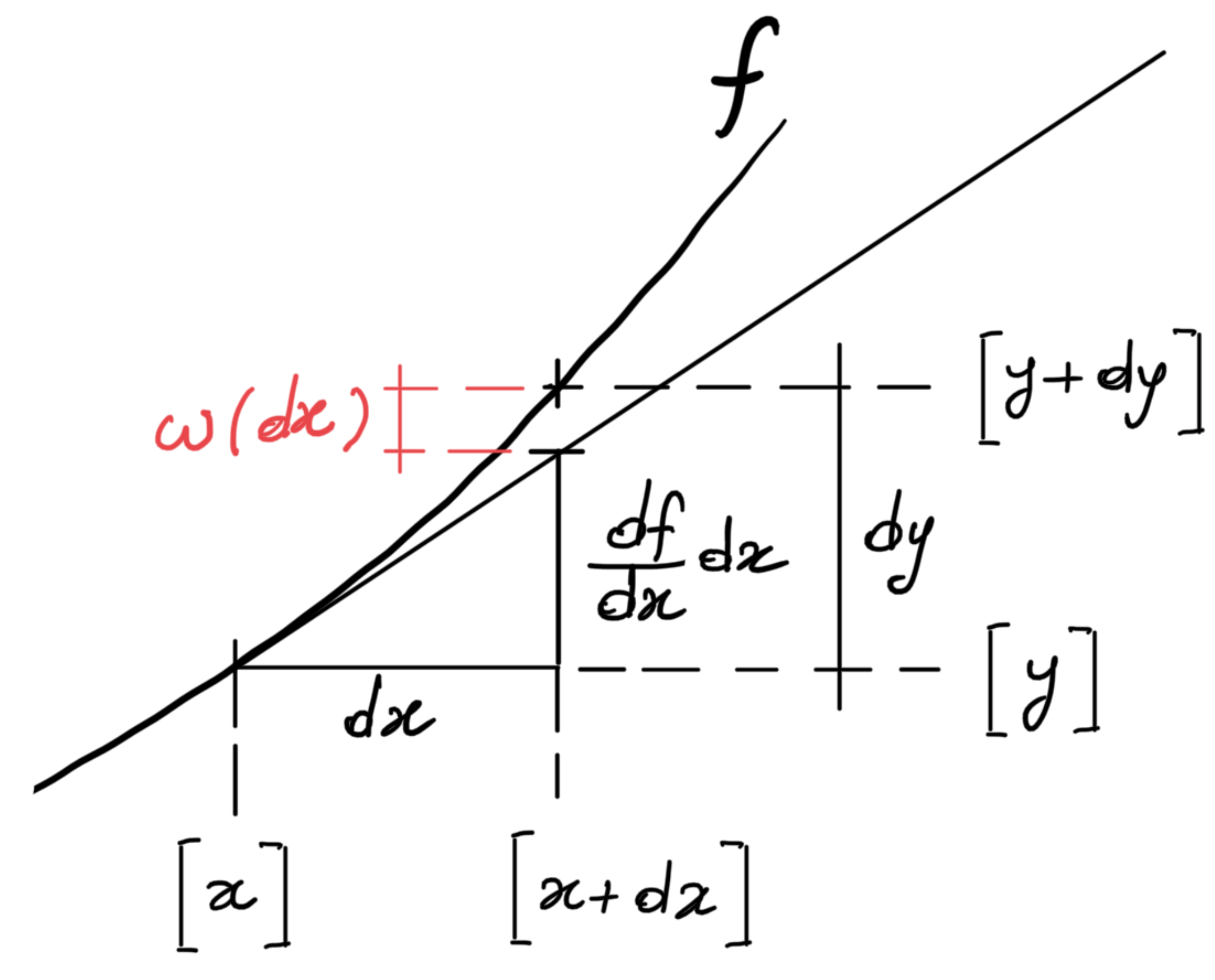
The transformation \(\vec{\chi}\) that was introduced to describe the motion of a body is completely generic therefore it is not necessarily linear. But we will see how this feature, linearity, still plays a fundamental role because, even if generic, \(\vec{\chi}\) can be described locally through its linearization. This idea is based on the notion of differential of a function.

In order to recall, in a simple way, the idea behind the linearization operations, this process is illustrated in the following figure for a real function depending on a single variable.

\begin{equation*} f \,:\, x \in \mathbb{R} \,\longmapsto\, y \in \mathbb{R} \end{equation*}

\begin{align*} dy \amp = \func{f}{x+dx} - \func{f}{x}\\ \amp = \func{f}{x} +\frac{df}{dx}\,dx + \func{\omega}{dx} - \func{f}{x}\\ \amp =\frac{df}{dx}\,dx + \func{\omega}{dx} \end{align*}

where \(\func{\omega}{dx}/dx \to 0\) if \(dx \to 0\text{,}\) then it is possible to state that

\begin{equation} dy = \frac{df}{dx}\,dx\,.\label{df_eq}\tag{1.3.1} \end{equation}

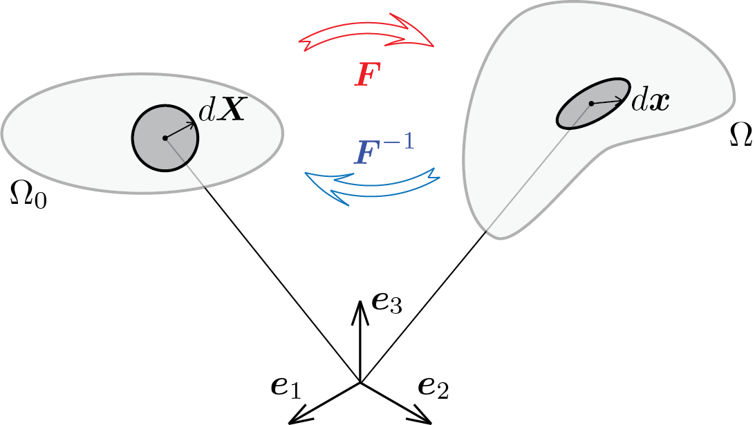
A rigorous generalization of the equation (1.3.1) would require additional instruments far beyond the introductory purposes of the present exposition. The final result is however given, result which provides the differential \(d\vec{x}\) relative to the current configuration as a function of the differential \(d\vec{X}\) relative to the reference configuration. For this purpose it si useful to write an expanded version of Equation (1.2.1)

The seeken differential can formulated as follows

These are a set of equations which can be expressed as multiplication between a matrix and a vector, i.e.

This result shows how the transition from \(d\vec{X}\) to \(d\vec{x}\) occurs through a linear transformation represented by the matrix \(\mat{F}\) which, for each point of the domain, contains all the information needed to characterize the deformation. \(\tens{F}\) is named as deformation gradient. On thsi basis the relationship between the differentials, \(d\vec{X}\) and \(d\vec{x}\text{,}\) can be expressed in compact form as

Relationship that can be specified more precisely as follows

where the dependence of \(\tens{F}\) on the point where the gradient is evaluated has been made explicit.

What is obtained for the transformation \(\vec{\chi} \) is also valid for its inverse \(\vec{\chi}^{-1}\text{,}\) therefore the following inverse relationship can be established between the differentials \(d\vec{X}\) and \(d\vec{x}\)

Typically the evaluation of the gradient of the inverse transformation does not pass through the explicit writing of \(\vec{\chi}^{- 1}\) but is done by calculating the inverse of \(\tens{F}\) for which invertibility must be ensured.

evaluation of the deformation gradient (nonlinear transformations).

In the case of nonlinear transformations it is not possible to identify a matrix associated with the transformation but, locally, the gradient of the transformation behaves like a linear transformation. Consider thus, for example, the transformation defined as

\begin{align*} x_1 \amp = \func{\chi_1}{X_1, X_2} = X_1^3\,,\\ x_2 \amp = \func{\chi_2}{X_1, X_2} = X_2^3\,. \end{align*}

The calculation of the partial derivatives gives

\begin{align*} \regulardiff{\chi_1}{X_1} = 3\,X_1^2\,,\amp\regulardiff{\chi_1}{X_2} = 0\,,\\ \regulardiff{\chi_2}{X_1} = 0\,,\amp\regulardiff{\chi_2}{X_2} = 3\,X_2^2 \end{align*}

allowing the evaluation of the deformation gradient

\begin{equation*} \func{\mat{F}}{\vec{X}} = \left[\begin{array}{cc} \regulardiff{\chi_1}{X_1} \amp \regulardiff{\chi_1}{X_2} \\ \regulardiff{\chi_2}{X_1} \amp \regulardiff{\chi_2}{X_2} \end{array}\right] = \left[\begin{array}{cc} 3\,X_1^2 \amp 0 \\ 0 \amp 3\,X_2^2 \end{array}\right] \end{equation*}

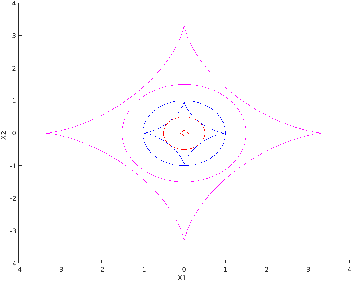
In order to visualize how the assigned transformation works let us consider, in the plane \((X_1, X_2)\text{,}\) three circumferences of radius \(0. \text{,}\) \(1.0\) and \(1.5\) and their configuratons obtained through the assigned nonlinear transformation. The MATLAB® instructions for the calculation and plotting of the circumferences in the reference configuration and in the current one are as reported below.

N=60;
angle=linspace(0,2*pi,N);

radius=1.0;
c1X=radius*cos(angle);
c1Y=radius*sin(angle);
c1x=c1X.^3;
c1y=c1Y.^3;

radius=0.5;
c2X=radius*cos(angle);
c2Y=radius*sin(angle);
c2x=c2X.^3;
c2y=c2Y.^3;

radius=1.5;
c3X=radius*cos(angle);
c3Y=radius*sin(angle);
c3x=c3X.^3;
c3y=c3Y.^3;

hold on
% circumference (r=1), reference and deformed configurations
plot(c1X,c1Y,'b-')
plot(c1x,c1y,'b-')

% circumference (r=0.5), reference and deformed configurations
plot(c2X,c2Y,'r-')
plot(c2x,c2y,'r-')

% circumference (r=1.5), reference and deformed configurations
plot(c3X,c3Y,'m-')
plot(c3x,c3y,'m-')

The previous instructions allow to obtain the following figure where the three circumferences, in the reference and current configurations, are represented with the colors red for the radius \(0.5\text{,}\) blue for the radius \(1.0\) and magenta for the radius \(1.5 \text{.}\)

For exercise and to compare the nonlinear transformation examined with simpler linear transformations, it is suggested to perform the same calculations for the Transformations 2, 3 and 4 discussed in the previous sections.