A first course on solid mechanics

Section 1.5 determinant of the deformation gradient

In previous sections tensors have been introduced as linear operators associated with linear transformations defined in the usual space \(\mathbb{R}^3\text{.}\) The use of the denomination linear operator instead of matrix indicates a mathematical object with a broader meaning but, in any case, the tensors share with matrices all the basic algebraic properties and operations. Therefore, in the following, speaking of matrices, some properties and operations will be resumed, such as the calculation of the determinant, placing them in the realm of the kinematic description of the bodies.

What is described in previous video lesson can be summarized as follows.

• The determinant is a real number which constitutes the scale factor of the areas, in the case of 2D transformations, or of the volumes, in the case of 3D transformations.
• From this perspective a null determinant is associated with transformations that scale to zero areas or volumes described in the initial space to which the transformation is applied. For example in 2D, the determinant is zero if all the points of the starting space are mapped on a line or, in the most extreme case, on a single point. In the 3D case, a transformation has zero determinant if it maps the points in a plane, in a straight line or in a single point. In these cases the columns of the matrix associated with the transformation are linearly dependent.
• The determinant can also be negative because it also carries information about a possible change of orientation of the area or of the starting volume. This occurs when the transformed vectors of the basis do not respect the right hand's rule.

Subsection 1.5.1 transformation formula of volume elements

Given the volume element \(dV = dX_1 dX_2 dX_3\) belonging to the reference configuration \(\body_0\text{,}\) it is possible to evaluate the corresponding volume element \(dv = dx_1 dx_2 dx_3 \) relative to the current configuration \(\body\text{.}\) The formula is

\begin{equation} dv = \func{J}{\vec{X}}\,dV\,,\label{volume_change_eq}\tag{1.5.1} \end{equation}

where

\begin{equation} \func{J}{\vec{X}} = \det{\func{\mat{F}}{\vec{X}}} > 0 \,.\tag{1.5.2} \end{equation}

Inequality highlights compliance with the following conditions: (i) due to the impenetrability of matter, transformations characterized by \(\func{J}{\vec{X},t} < 0\) are not admissible; (ii) the volumetric transformation ratio \(\func{J}{\vec{X}} = dv / dV \) cannot be null for any point \(\vec{X} \in \body_{0}\text{.}\) It is also possible to define the inverse volumetric ratio i.e.

\begin{equation} \func{J^{-1}}{\vec{x}} = \det{ \func{\mat{F}^{-1}}{\vec{x}} } > 0\,,\tag{1.5.3} \end{equation}

from which

\begin{equation} dV = \func{J^{-1}}{\vec{x}}\,dv\,.\label{inverse_volume_change_eq}\tag{1.5.4} \end{equation}

Transformations characterized by \(J = 1 \) will be called isochoric transformations.

calculation of the determinant of transformations and admissibility check.

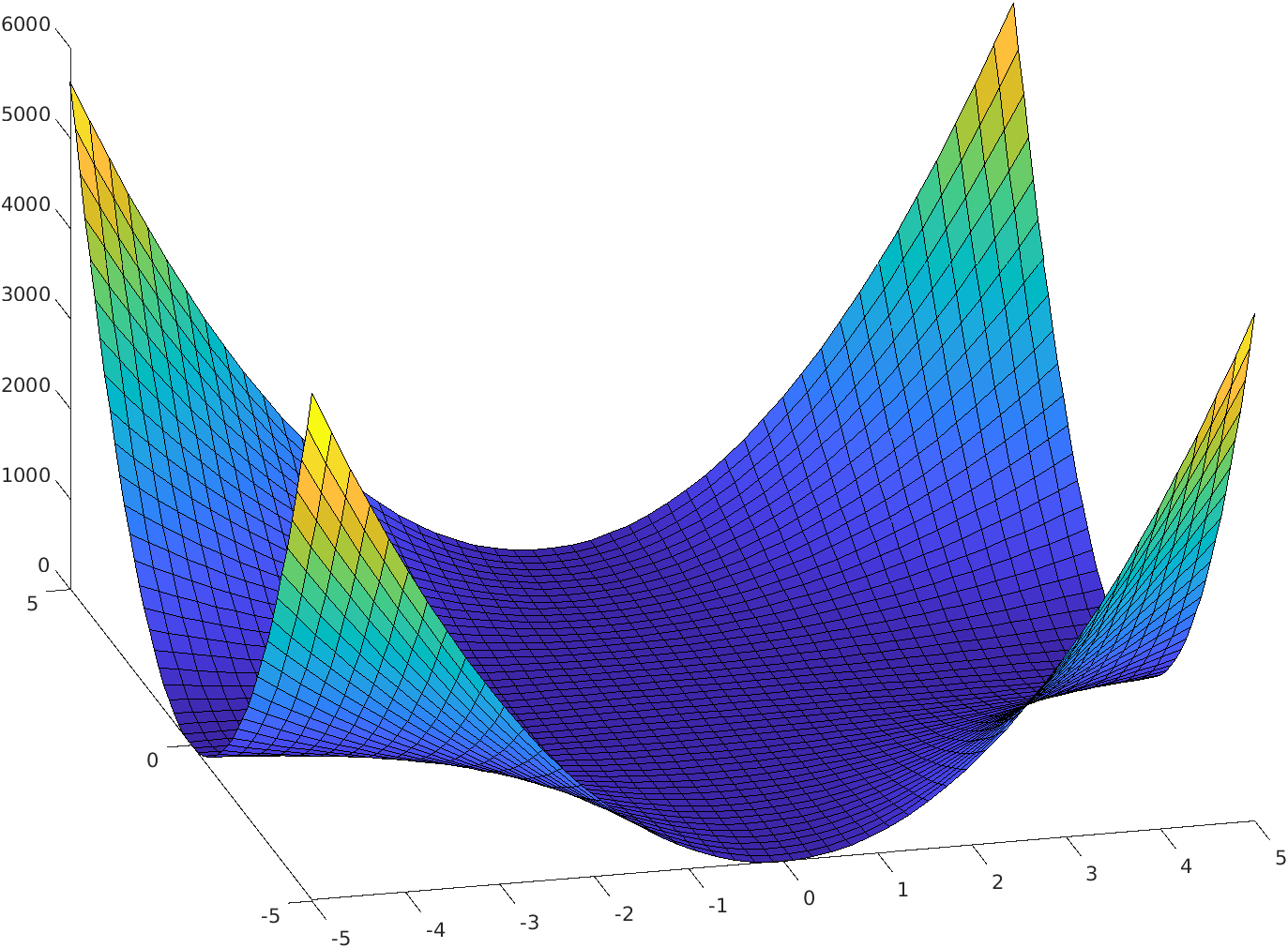
Considering the two-dimensional transformations considered in the previous examples, the following MATLAB® instructions are given to be used for the calculation of the determinant and for the verification of the admissibility of the transformation. The instructions for plotting the value of the determinant on the domain \(-5 < X_1 < 5\text{,}\) \(-5 < X_2 < 5\) are also given.

MATLAB® instructions for the Transformation 1.

T1 = @(X) [-X(2); X(1)];
F = [T1([1; 0]) T1([0; 1])];
syms detF(X1, X2);
detF(X1, X2) = det(F);

x = linspace(-5, 5, 50);
y = linspace(-5, 5, 50);
[X,Y] = meshgrid(x,y);

surface(X,Y,detF(X,Y))

Similar instructions can also be identified for Transformations 2, 3 and 4 which also verify the admissibility condition, being characterized by a determinant which is constant and greater than zero.

MATLAB® instructions for the transformation defined by \(x_1 = X_1^3\,,\; x_2 = X_2^3\text{.}\)

syms T1(X1, X2);
T1(X1, X2) = X1^3; 

syms T2(X1, X2);
T2(X1, X2) = X2^3; 

syms detF(X1, X2);
detF(X1,X2) = diff(T1, X1)*diff(T2, X2) - diff(T1, X2)*diff(T2, X1);

x = linspace(-5, 5, 50);
y = linspace(-5, 5, 50);
[X,Y] = meshgrid(x,y);

surface(X,Y,detF(X,Y))

The result of the previous instructions provides the following plot

plotting which can be used to verify that along the coordinated axes \(X_1 = 0 \) and \(X_2 = 0 \) the transformation has zero determinant and therefore is not admissible (remember in this regard the presence of cusps in the plots shown in Figure 1.3.4).