Section5.6application of static analysis to systems of bodies
Subsection5.6.1cantilever beam
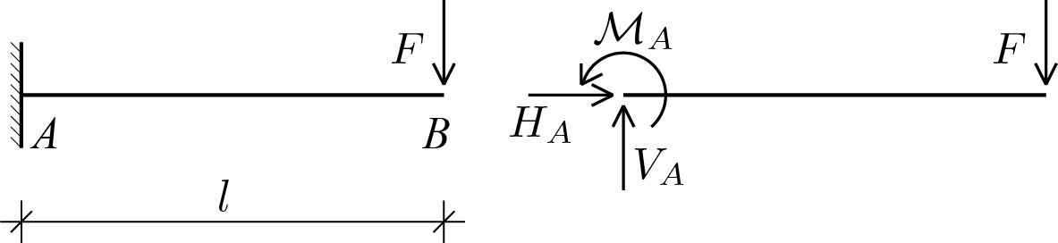
Consider a simple beam fixed at one end and subjected to a vertical force at the free end. The following figure shows the starting scheme and the free body diagram obtained by removing the fixed support and applying the related constraint reaction components (\(m = 3 \)).
The analysis involves only one body, therefore it is possible to write 3 equilibrium equations (\(n = 3 \)) which, taking as pole the end \(A \) in the rotational equilibrium of the beam, can be expressed as follows
\begin{align*}
H_A \amp = 0\,,\\
V_A - F \amp = 0\,,\\
\mathcal{M}_{A} - F l \amp = 0\,.
\end{align*}
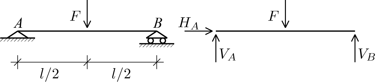
Consider a beam constrained in the manner shown in the figure and subjected to a vertical force in the middle. The same figure also shows the free body diagram obtained by removing the hinge and roller support and applying the related constraint reaction components (\(m = 3 \)).
The presence of a single body determines the writing of 3 equations of equilibrium (\(n = 3 \)) for which the extreme \(A \) is assumed as pole for rotational equilibrium:
\begin{align*}
H_A \amp = 0\,,\\
V_A + V_B - F \amp = 0\,,\\
V_{B} l - F l/2 \amp = 0\,.
\end{align*}
Also in this case the simple inspection of the static matrix allows to establish the isostaticity of the system. The calculation of the constraint reaction components provides:
$ % resultants' vector =
% [horizontal; vertical; torque]
R = zeros(3,1);

% function for the calculation of the moment
moment = @(X0, X, Load)...
    -Load(1)*(X(2)-X0(2))+Load(2)*(X(1)-X0(1));

% coordinates of the points on which the loads are applied
syms L;
A = [0; 0];
B = [L; 0];
C = [L/2; 0];

% choice of pole
POLE = A;

% for each point the vector Load = [F1; F2; M] is assigned
% and all the contribuitions are summed to R
syms HA VA;
LoadA = [HA; VA; 0];
R = R + LoadA;
R(3) = R(3) + moment(POLE, A, LoadA);
R

syms VB;
LoadB = [0; VB; 0];
R = R + LoadB;
R(3) = R(3) + moment(POLE, B, LoadB);
R

syms F;
CaricoC = [0; -F; 0];
R = R + LoadC;
R(3) = R(3) + moment(POLE, C, LoadC);
R

% equilibrium equations
eqns = [
R(1) ==0,
R(2) == 0,
R(3)==0
];

% static matrix and vector of the assigned loads
[B,b] = equationsToMatrix(eqns, [HA, VA, VB]);

% degrees of freedom, n
% constraint degrees, m
[n,m] = size(B);

% evaluation of the rank of B
r = rank(B);

% if the system is statically determined, the solution is calculated
if and(r == min(m,n), m == n)
    x = linsolve(B,b);
end

HA = x(1)
VA = x(2)
VB = x(3)
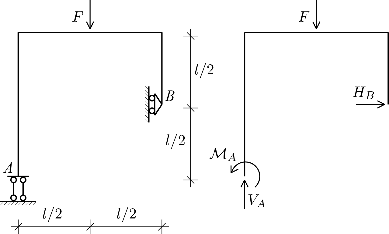
Consider the following simple frame subjected to a vertical force applied in the midle of the horizzontal beam. The constraints (\(m = 3 \)) are applied at the basis of the vertical beams and their removal and the subsequent application of the constraint reaction components leads to the free body diagram shown in the figure.
$ % resultants' vector =
% [horizontal; vertical; torque]
R = zeros(3,1);

% function for the calculation of the moment
moment = @(X0, X, Load)...
    -Load(1)*(X(2)-X0(2))+Load(2)*(X(1)-X0(1));

% coordinates of the points on which the loads are applied
syms L;
A = [0; 0];
B = [L; L/2];
C = [L/2; L];

% pole chosen
POLE = C;

% for each point the vector Load = [F1; F2; M] is assigned
% and all the contribuitions are summed to R
syms VA MA;
LoadA = [0; VA; MA];
R = R + LoadA;
R(3) = R(3) + moment(POLE, A, LoadA);
R

syms HB;
LoadB = [HB; 0; 0];
R = R + LoadB;
R(3) = R(3) + moment(POLE, B, LoadB);
R

syms F;
LoadC = [0; -F; 0];
R = R + LoadC;
R(3) = R(3) + moment(POLE, C, LoadC);
R

% equilibrium equations
eqns = [
R(1) ==0,
R(2) == 0,
R(3)==0
];

% static matrix and vector of the assigned loads
[B,b] = equationsToMatrix(eqns, [VA, MA, HB]);

% degrees of freedom, n
% constraint degrees, m
[n,m] = size(B);

% evaluation of the rank of B
r = rank(B);

% if the system is statically determined, the solution is calculated
if and(r == min(m,n), m == n)
    x = linsolve(B,b);
end

VA = x(1)
MA = x(2)
HB = x(3)
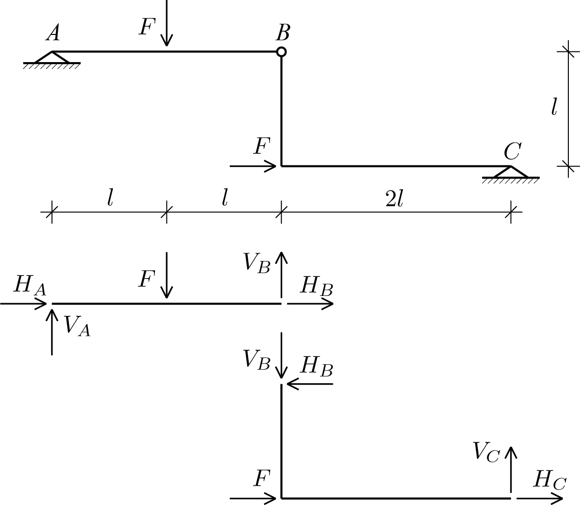
Consider the following system consisting of two bodies connected by an internal hinge. The removal of all the degrees of constraint (\(m = 6 \)) and the subsequent application of the constraint reaction components leads to the free body diagram shown in the figure.
The system consists of two bodies (\(n = 6 \)), allowing the writing of two groups of equations: the equilibrium equations for the body \(AB \) (pole in \(A \))
\begin{align*}
H_A + H_B \amp = 0\,,\\
V_A + V_B - F \amp = 0\,,\\
V_{B} 2l - F l \amp = 0\,,
\end{align*}
The calculation provides a rank equal to \(r = 6 \) which verifies the condition \(\text{min}(n, m) = 6 \text{.}\) Being \(m == n \) the system is isostatic. The linear system solution calculable with MATLAB®
$ % resultants' vector =
% [horizontal; vertical; torque]
% for the first body
R1 = zeros(3,1);
% and for the second body
R2 = zeros(3,1);

% function for the calculation of the moment
moment = @(X0, X, Load)...
    -Load(1)*(X(2)-X0(2))+Load(2)*(X(1)-X0(1));

% coordinates of the points on which the loads are applied
syms L;
A = [0; L];
B = [2*L; L];
C = [4*L; 0];
D = [L; L];
E = [2*L; 0];

% choosing pole for the first body
POLE = A;

% point A (first body)
syms HA VA;
LoadA = [HA; VA; 0];
R1 = R1 + LoadA;
R1(3) = R1(3) + moment(POLE, A, LoadA);

% point D (first body)
syms F;
LoadD = [0; -F; 0];
R1 = R1 + LoadD;
R1(3) = R1(3) + moment(POLE, D, LoadD);

% point B (first body)
syms HB VB;
LoadB = [HB; VB; 0];
R1 = R1 + LoadB;
R1(3) = R1(3) + moment(POLE, B, LoadB);

% choosing pole for the second body
POLE = B;

% point B (second body)
LoadB = [-HB; -VB; 0];
R2 = R2 + LoadB;
R2(3) = R2(3) + moment(POLE, B, LoadB);

% point E (second body)
LoadE = [F; 0; 0];
R2 = R2 + LoadE;
R2(3) = R2(3) + moment(POLE, E, LoadE);

% point C (second body)
syms HC VC;
LoadC = [HC; VC; 0];
R2 = R2 + LoadC;
R2(3) = R2(3) + moment(POLE, C, LoadC);

% equilibrium equations
eqns = [
R1(1) ==0,
R1(2) == 0,
R1(3)==0,
R2(1) ==0,
R2(2) == 0,
R2(3)==0
];

% static matrix and vector of the assigned loads
[B,b] = equationsToMatrix(eqns, [HA, VA, HB, VB, HC, VC]);

% degrees of freedom, n
% constraint degrees, m
[n,m] = size(B);

% evaluation of the rank of B
r = rank(B);

% if the system is statically determined, the solution is calculated
if and(r == min(m,n), m == n)
    x = linsolve(B,b);
end

HA = x(1)
VA = x(2)
HB = x(3)
VB = x(4)
HC = x(5)
VC = x(6)