
Section 3.1 motivation

In order to justify the need to introduce a constitutive modeling in our description of the mechanical behavior of solids under the action of the applied loads, we will consider a simple 1  case study and we will analyze it by using only what we have learned till now, i.e. Chapter 1 about the kinematics and Chapter 2 about statics.

simple means only that the analytical difficulties of finding a static solution are practically non-existent but the validity of what will be discussed remains absolutely general

Subsection 3.1.1 static analysis

Consider the following body with domain \(\body_0 \) delimited by the two end surfaces \(\Sigma_1 \) and \(\Sigma_2 \) and by the surface \(\Pi \) given by the other 4 faces of the prism. Let \(L \) be the length of the prism having a constant section along the axis and identified by the generic surface \(\Sigma \text{.}\) From a geometric point of view we will trivially have the following area and volume measurements

\begin{equation*} \func{A}{\Sigma} = \func{A}{\Sigma_1} = \func{A}{\Sigma_2} = S\,,\qquad \func{V}{\body_0} = L \, \func{A}{\Sigma} = L\, S\,, \end{equation*}

where \(S\) is the area of surface \(\Sigma\) which identifies the generic section of the prism. The bulk load is zero, \(\vec{b} = \vec{0} \text{,}\) and suppose that the prism is subject only to the tractions shown in the figure, tractions which are equal and opposite.

Figure 3.1.1.
Remark 3.1.2. very important assumption.

The geometric description just given concerns only the reference configuration \(\body_0 \) to which the kinematic description of the bodies typically refers, as presented in the Chapter 1. The writing of equilibrium equations, see in this regard the Chapter 2, is instead carried out with respect to the current configuration \(\body \text{.}\) The following discussion should therefore take account of this situation, also requiring the introduction of further concepts that are outside the present introductory discussion on Solid Mechanics.

Therefore we introduce the hypothesis behind a linearized formulation of the elastic problem, which is the final objective of this chapter, namely that equilibrium equations can be formulated assuming

\begin{equation} \body \equiv \body_0 \label{elasticity_basic_assumption_eq}\tag{3.1.1} \end{equation}
given the smallness of the displacements and deformations involved in the problem. Consequently also all operations, for example derivation and integration, will be carried out with respect to the coordinates \(X_1 \text{,}\) \(X_2 \) and \(X_3 \) related to the configuration of reference, or undeformed configuration, of the body.

Based on the data of the problem and the previous hypothesis, the static problem assumes the following formulation.

  • Equilibrium equations over the domain
    \begin{equation} \text{div}\tens{\sigma} = \vec{0}\quad\;\text{in}\;\body_0\,.\label{motiv_static_eq}\tag{3.1.2} \end{equation}
    That is, for components, the following three scalar equations
    \begin{equation} \begin{array}{l} \frac{\partial\sigma_{11}}{\partial X_1} + \frac{\partial\sigma_{12}}{\partial X_2} + \frac{\partial\sigma_{13}}{\partial X_3} = 0\\ \frac{\partial\sigma_{12}}{\partial X_1} + \frac{\partial\sigma_{22}}{\partial X_2} + \frac{\partial\sigma_{23}}{\partial X_3} = 0\\ \frac{\partial\sigma_{13}}{\partial X_1} + \frac{\partial\sigma_{23}}{\partial X_2} + \frac{\partial\sigma_{33}}{\partial X_3} = 0 \end{array} \quad\;\text{in}\;\body_0\,.\label{motiv_static_components_eq}\tag{3.1.3} \end{equation}
  • Static conditions on the boundary
    \begin{align} \amp \tens{\sigma}\vec{n}_1 = \vec{t}_1\quad\;\text{su}\;\Sigma_1 \,,\label{motiv_bc1_eq}\tag{3.1.4}\\ \amp \tens{\sigma}\vec{n}_2 = \vec{t}_2\quad\;\text{su}\;\Sigma_2 \,,\label{motiv_bc2_eq}\tag{3.1.5}\\ \amp \tens{\sigma}\vec{n}_{\Pi} = \vec{0}\quad\;\text{su}\;\Pi \,.\label{motiv_bc3_eq}\tag{3.1.6} \end{align}
    Where
    \begin{align} \Sigma_1:\amp \quad \matWp{n}{1} = \left[\begin{array}{r}0\\0\\-1\end{array}\right]\,,\;\matWp{t}{1} = \left[\begin{array}{r}0\\0\\-\bar{t}\end{array}\right] \,,\tag{3.1.7}\\ \Sigma_2:\amp \quad \matWp{n}{2} = \left[\begin{array}{r}0\\0\\1\end{array}\right]\,,\;\matWp{t}{2} = \left[\begin{array}{r}0\\0\\\bar{t}\end{array}\right] \,,\tag{3.1.8}\\ \Pi:\amp \quad \matWp{n}{\Pi} = \left[\begin{array}{r}n_1\\n_2\\0\end{array}\right] \,.\tag{3.1.9} \end{align}

Subsubsection 3.1.1.1 stress field assumption and solution

In Eq. (3.1.2) the unknowns are the 6 independent components of the stress tensor while the equations available are only 3. Put in these terms the search for the solution would not even be possible. However, given the simplicity of the data of the problem, it is possible to assume a form the stress tensor field and check if all equilibrium equations, over the domain and on the boundary, are satisfied. In particular, let us consider the following form for \(\tens{\sigma} \)

\begin{equation} \mat{\sigma} = \left[\begin{array}{ccc} 0 \amp 0 \amp 0\\ 0 \amp 0 \amp 0\\ 0 \amp 0 \amp \kappa \end{array}\right]\tag{3.1.10} \end{equation}

valid on the whole domain and with \(\kappa \) a generic constant. The satisfaction of Eq. (3.1.3) is easily verified:

\begin{equation*} \begin{array}{l} \frac{\partial\, 0}{\partial\, X_1} + \frac{\partial\, 0}{\partial\, X_2} + \frac{\partial\, 0}{\partial\, X_3} = 0\\ \frac{\partial\, 0}{\partial\, X_1} + \frac{\partial\, 0}{\partial\, X_2} + \frac{\partial\, 0}{\partial\, X_3} = 0\\ \frac{\partial\, 0}{\partial\, X_1} + \frac{\partial\, 0}{\partial\, X_2} + \frac{\partial\, \kappa}{\partial\, X_3} = 0 \end{array} \quad\;\text{in}\;\body_0\,. \end{equation*}

The satisfaction of Eq. (3.1.6) can be also easily verified:

\begin{equation*} \left[\begin{array}{ccc} 0 \amp 0 \amp 0\\ 0 \amp 0 \amp 0\\ 0 \amp 0 \amp \kappa \end{array}\right] \left[\begin{array}{r}n_1\\n_2\\0\end{array}\right] = \left[\begin{array}{r}0\\0\\0\end{array}\right] \,. \end{equation*}

While imposing Eq. (3.1.4), or Eq. (3.1.5), it can be obtained what follows

\begin{equation*} \left[\begin{array}{ccc} 0 \amp 0 \amp 0\\ 0 \amp 0 \amp 0\\ 0 \amp 0 \amp \kappa \end{array}\right] \left[\begin{array}{r}0 \\ 0\\-1\end{array}\right] = \left[\begin{array}{r}0\\0\\-\bar{t}\end{array}\right] \quad \rightarrow \quad \kappa = \bar{t} \,. \end{equation*}

Ultimately the stress field which satisfies all equilibrium quations involved is

\begin{equation} \mat{\sigma} = \left[\begin{array}{ccc} 0 \amp 0 \amp 0\\ 0 \amp 0 \amp 0\\ 0 \amp 0 \amp \bar{t} \end{array}\right]\,.\label{motiv_static_solution_eq}\tag{3.1.11} \end{equation}

Therefore the static solution is given by a state of pure traction along the \(X_3 \) axis distributed evenly over the whole body.

Subsection 3.1.2 kinematic analysis

Based on what we learned in Chapter 1 and what we got as a static solution, we are able to speculate a quite plausible kinematic transformation for the problem under consideration. For example, consider what is shown in the following figure.

Figure 3.1.3.

The represented trasnformation is

\begin{align} x_1 \amp = \func{\chi_1}{X_1, X_2, X_3} = X_1\,,\label{motiv_kinematic_solution1_eq}\tag{3.1.12}\\ x_2 \amp = \func{\chi_3}{X_1, X_2, X_3} = X_2\,,\label{motiv_kinematic_solution2_eq}\tag{3.1.13}\\ x_3 \amp = \func{\chi_3}{X_1, X_2, X_3} = \lambda\,X_3\,,\label{motiv_kinematic_solution3_eq}\tag{3.1.14} \end{align}

where \(\lambda\) is a generic parameter to be determined. The displacement field \(\vec{u}\) has the following components

\begin{align} u_1 \amp = x_1 - X_1 = 0\,,\label{motiv_displ_solution1_eq}\tag{3.1.15}\\ u_2 \amp = x_2 - X_2 = 0\,,\label{motiv_displ_solution2_eq}\tag{3.1.16}\\ u_3 \amp = x_3 - X_3 = (\lambda - 1)X_3\,,\label{motiv_displ_solution3_eq}\tag{3.1.17} \end{align}

and its gradient is

\begin{equation} \mat{\nabla u} = \left[\begin{array}{ccc} \regulardiff{u_1}{X_1} \amp \regulardiff{u_1}{X_2} \amp \regulardiff{u_1}{X_3}\\ \regulardiff{u_2}{X_1} \amp \regulardiff{u_2}{X_2} \amp \regulardiff{u_2}{X_3}\\ \regulardiff{u_3}{X_1} \amp \regulardiff{u_3}{X_2} \amp \regulardiff{u_3}{X_3} \end{array}\right] = \left[\begin{array}{ccc} 0 \amp 0 \amp 0\\ 0 \amp 0 \amp 0\\ 0 \amp 0 \amp (\lambda - 1) \end{array}\right]\,.\tag{3.1.18} \end{equation}

As for the kinematic description of the problem, we are unable to add anything else. So let's see if using another tool introduced in Chapter 2, the Principle of virtual work, it is possible to gain some kind of information on the generic parameter \(\lambda \text{.}\)

Subsection 3.1.3 Principle of virtual work

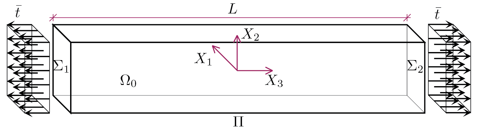
On the basis of the displacement field adopted, the data of the problem under examination and the basic assumption (3.1.1), the writing of the Principle of virtual work (2.5.5) takes the following expression

\begin{equation} \underbrace{\int_{\Sigma_1} \vec{t}_1 \cdot \vec{u}_1\,dS + \int_{\Sigma_2} \vec{t}_2 \cdot \vec{u}_2\,dS}_{\text{L}_{\text{est}}} = \underbrace{\int_{\body_0} \tens{\sigma} : \text{sym}\tens{\nabla u}\,dV}_{\text{L}_{\text{int}}}\,,\label{motiv_plv_eq}\tag{3.1.19} \end{equation}

where, in particular,

\begin{equation*} 
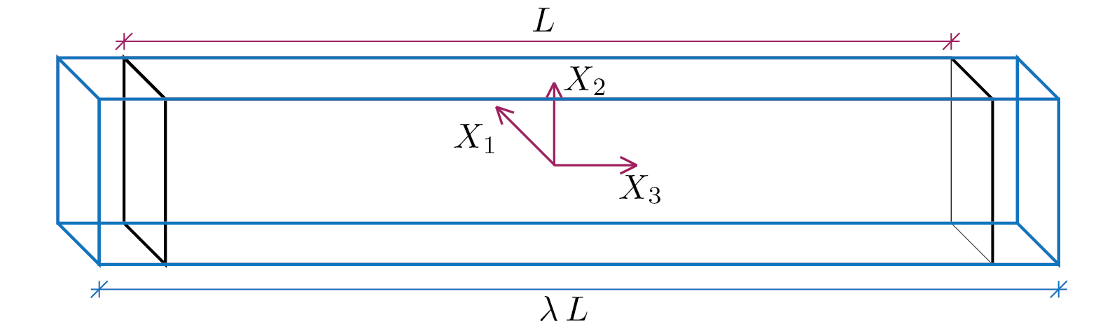
\matWp{u}{1} = \left[\begin{array}{c}0\\0\\-(\lambda - 1)\frac{L}{2}\end{array}\right]\,,\; \matWp{u}{2} = \left[\begin{array}{c}0\\0\\(\lambda - 1)\frac{L}{2}\end{array}\right]\,,\; \text{sym}\tens{\nabla u} = \tens{\nabla u}\,. \end{equation*}

Then introducing the static solution already found and the expression above reported of the gradient of the displacement the following result is obtained

\begin{equation} \int_{\Sigma_1} \bar{t}\,(\lambda - 1)\frac{L}{2} \,dS + \int_{\Sigma_2} \bar{t}\,(\lambda - 1)\frac{L}{2} \,dS = \int_{\body_0} \bar{t}\,(\lambda - 1) \,dV\,.\tag{3.1.20} \end{equation}

From which, evaluating the involved integrals (all with constant argument), it can be obtained what follows

\begin{equation} \bar{t}\,(\lambda - 1)\frac{L}{2}\,S + \bar{t}\,(\lambda - 1)\frac{L}{2}\,S = \bar{t}\,(\lambda - 1)\,\,S\,L\,,\tag{3.1.21} \end{equation}

i.e.

\begin{equation} \underbrace{\bar{t}\,(\lambda - 1)\,\,L\,S}_{\text{L}_{\text{est}}} = \underbrace{\bar{t}\,(\lambda - 1)\,\,S\,L}_{\text{L}_{\text{int}}}\,,\tag{3.1.22} \end{equation}

Therefore it is also possible to verify the equality between external and internal work but we do not draw any further information regarding the \(\lambda \) parameter.

Subsection 3.1.4 conclusions

Previous discussion allows to draw the following conclusions.

  1. It was possible to identify the tensor \(\sigma \) which satisfies the equilibrium equations.  2 .
  2. We have identified a displacement field parameterized with respect to the \(\lambda \) parameter, a plausible field and which also verifies the Principle of virtual work.
  3. It is not possible, at least with the tools available so far, to find a significative value for \(\lambda \) from a mechanical point of view. This parameter remains completely generic and undefined.
  4. Even the form assumed for the transformation (3.1.12) - (3.1.14) has not been subject to verification and at the moment remains completely arbitrary.
This result was made possible only by the problem under examination, a very particular problem which therefore does not constitute a typical situation. In general, equilibrium equations are not solvable with respect to the components of the stress tensor.

The problem highlighted depends on a lack of information in the mechanical model presented so far. The missing information is as follows

In the following sections this problem is presented and discussed, not in the most general terms possible, but with respect to the context already largely used for the problem examined above. That is, in the context of small displacements and small strains also known as infinitesimal displacements context. Therefore a link will be established between the Cauchy stress tensor and the infinitesimal strain tensor:

\begin{equation} \tens{\sigma} = \func{\tens{\sigma}}{\tens{\varepsilon}}\,.\tag{3.1.23} \end{equation}

It is useful to poit out that, in the case of infinitesimal displacements, the infinitesimal strain tensor constitutes an approximation of the Green-Lagrange strain tensor, see Section 1.9, and that in the calculation of internal work this tensor appears too. Indeed

\begin{equation} \text{L}_{\text{int}} = \int_{\body_0} \tens{\sigma} : \text{sym}\tens{\nabla u}\,dV = \int_{\body_0} \tens{\sigma} : \tens{\varepsilon}\,dV\,.\tag{3.1.24} \end{equation}