
Section 5.8 2D beam equilibrium differential equations

The equilibrium equations for the beam have already been presented in Section 3.5 and Section 3.6 in the broader context which led to the construction of a complete 2D elastic beam model. Here the equations are obtained by other means, moreover the shear force is taken into account in a explict way.

Subsection 5.8.1 formulation of the problem

Figure 5.8.1.

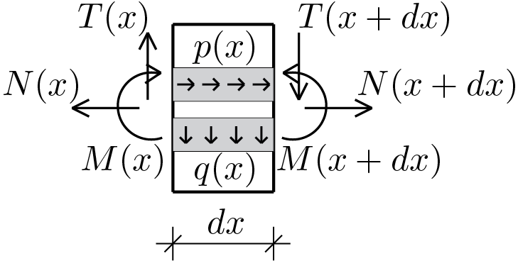
Let us consider a beam subjected to generic loading conditions, let us assume to isolate a portion of the beam with infinitesimal length \(dx\text{.}\) The beam's portion thus identified is subjected to a series of actions shown in the figure and which, for clarity, are listed below:

  • generalized section forces, \(N(x)\text{,}\) \(T(x)\) e \(M(x)\text{,}\) relative to point \(x\) along the beam axis;
  • generalized section forces, \(N(x+dx)\text{,}\) \(T(x+dx)\) e \(M(x+dx)\text{,}\) relative to point \(x+dx\text{;}\)
  • axial distributed load \(p(x)\text{;}\)
  • transverse distributed load \(q(x)\text{.}\)

Subsection 5.8.2 equilibrium conditions

The obtained scheme is essentially a free body diagram for which it is possible to impose the following equations of equilibrium (the pole used for the rotational equilibrium is placed at the abscissa \(x + dx \))

\begin{align} -N(x) + N(x+dx) + p(x)dx \amp = 0\,,\tag{5.8.1}\\ -T(x) + T(x+dx) + q(x)dx \amp = 0\,,\tag{5.8.2}\\ -T(x)\,dx - M(x) + q(x)\frac{dx^2}{2} + M(x+dx) \amp = 0\,.\tag{5.8.3} \end{align}

The hypothesis of continuity of the one-dimensional solid and of the quantities defined on it, allows to use Taylor series truncated to the first order of the generalized section forces evaluated on the section \(x + dx \) and to obtain therefore

\begin{align} -N(x) + \underbrace{N(x) + \frac{d N}{d x}\,dx}_{N(x+dx)} + p(x)dx \amp = 0\,,\tag{5.8.4}\\ -T(x) + \underbrace{T(x) + \frac{d T}{d x}\,dx}_{T(x+dx)} + q(x)dx \amp = 0\,,\tag{5.8.5}\\ -T(x)\,dx - M(x) + q(x)\frac{dx^2}{2} + \underbrace{M(x) + \frac{d M}{d x}\,dx}_{M(x+dx)} \amp = 0\,.\tag{5.8.6} \end{align}

where the quantities \(\frac{d N}{d x} \text{,}\) \(\frac{d T}{d x} \) and \(\frac{d M}{d x} \) denote the derivatives of the generalized section forces with respect to the abscissa \(x \text{.}\) Making the necessary simplifications and neglecting the term \(q(x)\frac{dx^2}{2} \) because of higher order than the first, we obtain the equilibrium differential equations for the 2D beam listed below .

  • Axial direction equilibrium:
    \begin{equation} \frac{d N}{d x} + p(x) = 0\,.\tag{5.8.7} \end{equation}
  • Transverse direction equilibrium:
    \begin{equation} \frac{d T}{d x} + q(x) = 0\,.\tag{5.8.8} \end{equation}
  • Rotational equlibrium:
    \begin{equation} \frac{d M}{d x} - T = 0\,.\tag{5.8.9} \end{equation}

Subsection 5.8.3 general integrals

The integration of the equilibrium differential equations gives the following general integrals valid on portions of beam along which the generalized section forces are analytic in the variable \(x\text{:}\)

\begin{align} N(x) \amp = -\int p(x) dx + a \,,\label{general_N_eq}\tag{5.8.10}\\ T(x) \amp = -\int q(x) dx + b \,,\label{general_T_eq}\tag{5.8.11}\\ M(x) \amp = \int\left(-\int q(x) dx\right)dx + b\,x + c \,.\label{general_M_eq}\tag{5.8.12} \end{align}

The integration constants \(a \text{,}\) \(b \) and \(c \) are to be evaluated on the basis of the assigned boundary conditions.

\(p(x)=0\) and \(q(x)=0\) case.

In order to illustrate the evaluation of the integration constants, consider the following free body diagram.

Figure 5.8.2.

For the absence of distributed loads the general integrals give

\begin{align*} N(x) \amp = a \,,\\ T(x) \amp = b \,,\\ M(x) \amp = b\,x + c \,. \end{align*}

Therefore we have a constant pattern for \(N \) and \(T \) and linear for \(M \text{.}\) By imposing the boundary conditions

\begin{equation*} N(0) = F\,,\quad T(0) = F\,, \quad M(0) = -Fl\,, \end{equation*}

it can be obtained

\begin{equation*} a = F\,,\quad b = F\,, \quad c = -Fl\,. \end{equation*}

Then the analytical expression of the generalized section forces becomes

\begin{align*} N(x) \amp = F \,,\\ T(x) \amp = F \,,\\ M(x) \amp = F\,x - Fl \,. \end{align*}

The same result would have been obtained using the boundary conditions

\begin{equation*} N(l) = F\,,\quad T(l) = F\,, \quad M(l) = 0\,. \end{equation*}

Subsection 5.8.4 general integrals for constant distributed loads

Figure 5.8.3.

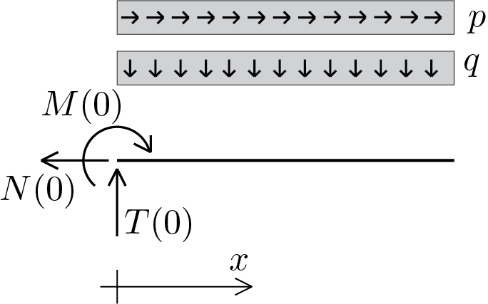
The diagram shows the case of a beam of which the values of the stress components at the extreme \(x = 0 \) are known and is subjected to constant distributed loads. In this case the general integrals (5.8.10), (5.8.11) and (5.8.12) take the following expressions

\begin{align} N(x) \amp = -p\,x + N(0) \,,\label{general_const_N_eq}\tag{5.8.13}\\ T(x) \amp = -q\,x + T(0) \,,\label{general_const_T_eq}\tag{5.8.14}\\ M(x) \amp = -q \frac{x^2}{2} + T(0)\,x + M(0) \,.\label{general_const_M_eq}\tag{5.8.15} \end{align}

Expressions showing a linear pattern for axial and shear forces and a parabolic pattern for the bending moment.