the elastic problem

Section 3.4 the elastic problem

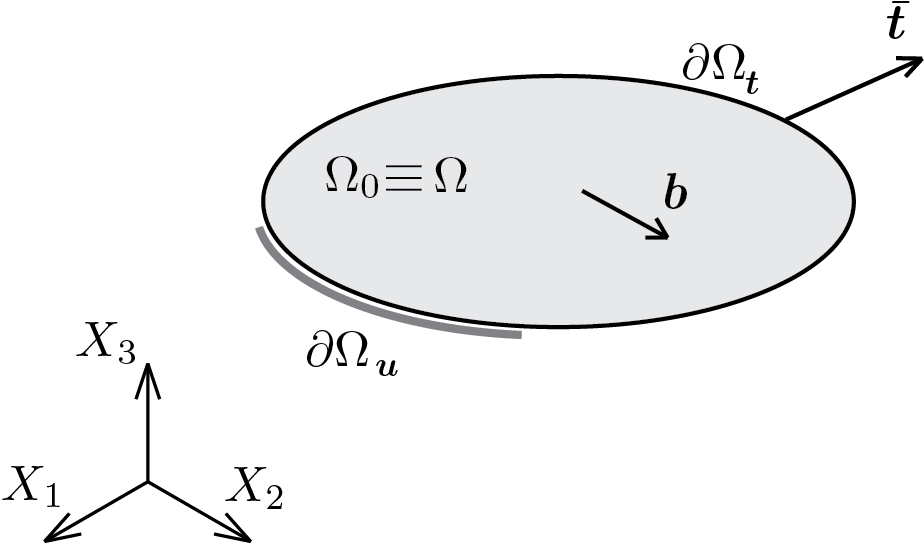
The definition of the elastic law provided in the previous sections allows to formulate, in well-posed terms, the following problem known as elastic problem.

🔗

Evaluation of the displacement, stress and strain fields, \(\vec{u}\text{,}\) \(\tens{\sigma}\) and \(\tens{\varepsilon}\text{,}\) caused by the assigned loading conditions on a body \(\body\) however constrained.

🔗

Answering the question posed requires the simultaneous solution of the following equations defined on all points of the assigned body \(\body \text{.}\)

🔗

Equilibrium equations (Chapter 2)
\begin{equation} \text{div}\tens{\sigma} + \vec{b} = \vec0\,.\tag{3.4.1} \end{equation}

🔗
Strain-displacement relationship (Chapter 1)
\begin{equation} \tens{\varepsilon} = \text{sym}\tens{\nabla u}\,.\tag{3.4.2} \end{equation}

🔗
Elastic constitutive law (Chapter 3)
\begin{equation} \tens{\sigma} = \tensQ{C}:\tens{\varepsilon}\,.\tag{3.4.3} \end{equation}

🔗

🔗

To complete the formulation of the problem it is also necessary to assign the boundary conditions which, in general, can be of two types: static type on the part of boundary \(\partial\body_{\vec{t}}\) and kinematic type on the part \(\partial\body_{\vec{u}}\text{.}\) Note \(\partial\body=\partial\body_{\vec{u}}+\partial\body_{\vec{t}}\text{.}\)

Static boundary conditions, defined on \(\partial\body_{\vec{t}}\)
\begin{equation} \tens{\sigma}\,\vec{n} = \bar{\vec{t}}\,.\tag{3.4.4} \end{equation}

🔗
Kinematic boundary conditions, defined on \(\partial\body_{\vec{u}}\)
\begin{equation} \vec{u} = \bar{\vec{u}}\,.\tag{3.4.5} \end{equation}

🔗

🔗

Subsection 3.4.1 motivation (reprised): the prismatic solid simply stretched

It is now possible to consider again the prismatic solid simply stretched discussed in Section 3.1 at the beginning of this chapter.

🔗

The static solution already found, however correct because it satisfies the equations of equilibrium (3.4.1) inside the solid and the static conditions on the contour (3.4.4), is

\begin{equation} \sigma_{11} = \sigma_{22} = \sigma_{12} = \sigma_{13} = \sigma_{23} = 0\,\quad \sigma_{33} = \bar{t}\,.\tag{3.4.6} \end{equation}

On the basis of the isotropic elastic relationship (3.3.11), it is now possible to calculate the strain tensor whose only non-null components are

\begin{align} \amp \varepsilon_{33} = \frac{\sigma_{33}}{E} = \frac{\bar{t}}{E}\,,\tag{3.4.7}\\ \amp \varepsilon_{22} = -\nu\,\varepsilon_{33} = -\nu\,\frac{\bar{t}}{E}\,,\tag{3.4.8}\\ \amp \varepsilon_{11} = -\nu\,\varepsilon_{33} = -\nu\,\frac{\bar{t}}{E}\,,\tag{3.4.9} \end{align}

therefore a constant and homogeneous strain field on the whole solid.

🔗

The strain-displacement relationship (3.4.2) allows the determination of the displacement field. An explicit writing of Eq. (3.4.2), see also (1.9.4), gives

\begin{align*} \varepsilon_{11} = \frac{\partial u_1}{\partial X_1}\,,\amp\qquad \varepsilon_{23} = \frac{1}{2}\left(\frac{\partial u_2}{\partial X_3} + \frac{\partial u_3}{\partial X_2}\right)\,,\\ \varepsilon_{22} = \frac{\partial u_2}{\partial X_2}\,,\amp\qquad \varepsilon_{31} = \frac{1}{2}\left(\frac{\partial u_3}{\partial X_1} + \frac{\partial u_1}{\partial X_3}\right)\,,\\ \varepsilon_{33} = \frac{\partial u_3}{\partial X_3}\,,\amp\qquad \varepsilon_{12} = \frac{1}{2}\left(\frac{\partial u_1}{\partial X_2} + \frac{\partial u_2}{\partial X_1}\right)\,. \end{align*}

By replacing the values of the strain components obtained in (3.4.7) - (3.4.9) by means of the elastic law we obtain

\begin{align} -\nu\,\frac{\bar{t}}{E}\ = \frac{\partial u_1}{\partial X_1}\,,\amp\qquad 0 = \frac{1}{2}\left(\frac{\partial u_2}{\partial X_3} + \frac{\partial u_3}{\partial X_2}\right)\,,\tag{3.4.10}\\ -\nu\,\frac{\bar{t}}{E}= \frac{\partial u_2}{\partial X_2}\,,\amp\qquad 0 = \frac{1}{2}\left(\frac{\partial u_3}{\partial X_1} + \frac{\partial u_1}{\partial X_3}\right)\,,\tag{3.4.11}\\ \frac{\bar{t}}{E} = \frac{\partial u_3}{\partial X_3}\,,\amp\qquad 0 = \frac{1}{2}\left(\frac{\partial u_1}{\partial X_2} + \frac{\partial u_2}{\partial X_1}\right)\,.\tag{3.4.12} \end{align}

Equations for which it is easy to verify that a solution is given by

\begin{equation} u_1 = -\nu\,\frac{\bar{t}}{E} \, X_1\,,\quad u_2 = -\nu\,\frac{\bar{t}}{E} \, X_2\,,\quad u_3 = \frac{\bar{t}}{E} \, X_3\,.\tag{3.4.13} \end{equation}

In this regard, it is observed that we say a solution since by adding to this displacement field all possible rigid motions, which in the assigned problem are not explicitly eliminated, we would always obtain the same solution in terms of stress and strain fields.

🔗

check.

Based on the displacement field defined by the (3.4.13) use the following MATLAB® instructions to calculate the relative strain and stress fields.

Listing 3.4.2.

🔗

$ syms t E ni;
X = sym('X', [1 3]);
u = sym('u', [1 3]);
u(1) = -ni*t/E * X(1);
u(2) = -ni*t/E * X(2);
u(3) = t/E * X(3);

Du = [transpose(gradient(u(1), X)); ...
transpose(gradient(u(2), X)); transpose(gradient(u(3), X))];

symDu = 1/2*(Du+transpose(Du))

Voigt_eps = [symDu(1,1); symDu(2,2); symDu(3,3); ...
2*symDu(2,3); 2*symDu(3,1); 2*symDu(1,2)];

Voigt_C = E/((1+ni)*(1-2*ni))*[(1-ni) ni ni 0 0 0; ...
 ni (1-ni) ni 0 0 0; ...
 ni ni (1-ni) 0 0 0; ...
 0 0 0 (1-2*ni)/2 0 0; ...
 0 0 0 0 (1-2*ni)/2 0; ...
 0 0 0 0 0 (1-2*ni)/2];

Voigt_sig = Voigt_C*Voigt_eps;
simplify(Voigt_sig)

🔗

Subsection 3.4.2 the prismatic solid simply bent

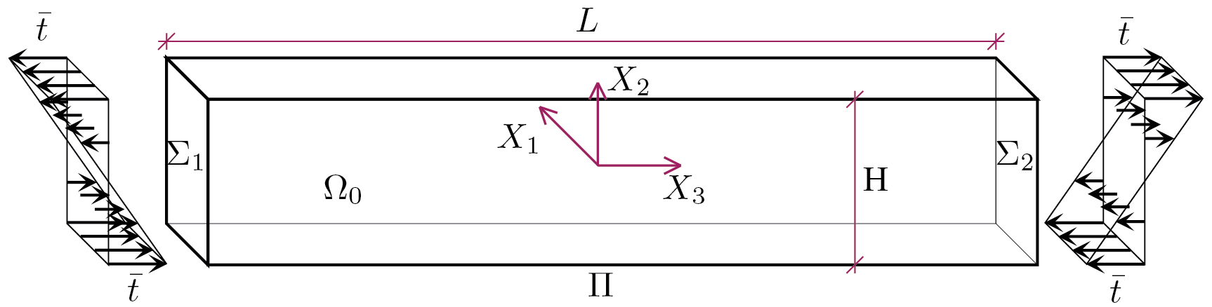
What has been obtained for the prismatic solid subject to uniform traction fields at the ends can be easily extended to the case in which the tractions applied to the ends have the linear trend shown in the following figure.

🔗

Subsubsection 3.4.2.1 static analysis

The formulation of the static part of the problem is identical to that made for the prismatic solid simply stretched except for the end faces of the solid on which the applied tractions assume the following expression

\begin{align} \Sigma_1:\amp\quad \matWp{t}{1} = \left[\begin{array}{c}0\\0\\-\frac{\bar{t}}{H/2}\,X_2\end{array}\right] \,,\tag{3.4.14}\\ \Sigma_2:\amp\quad \matWp{t}{2} = \left[\begin{array}{c}0\\0\\\frac{\bar{t}}{H/2}\,X_2 \end{array}\right] \,,\tag{3.4.15} \end{align}

where \(H \) represents the height of the solid along the direction \(X_2 \) and \(\bar{t} \) is the maximum intensity of the applied tractions.

🔗

Also in this case it is possible to proceed by assuming an attempt solution for the stress tensor and then verifying the satisfaction of the equations of equilibrium and of the boundary conditions. In particular for \(\tens{\sigma} \) the following form is assumed

\begin{equation} \mat{\sigma} = \left[\begin{array}{ccc} 0 \amp 0 \amp 0\\ 0 \amp 0 \amp 0\\ 0 \amp 0 \amp \kappa\,X_2 \end{array}\right]\tag{3.4.16} \end{equation}

valid on the whole domain and with \(\kappa \) a generic constant. With such an assumption the writing of balance equations provides

\begin{equation*} \begin{array}{l} \frac{\partial\, 0}{\partial\, X_1} + \frac{\partial\, 0}{\partial\, X_2} + \frac{\partial\, 0}{\partial\, X_3} = 0\\ \frac{\partial\, 0}{\partial\, X_1} + \frac{\partial\, 0}{\partial\, X_2} + \frac{\partial\, 0}{\partial\, X_3} = 0\\ \frac{\partial\, 0}{\partial\, X_1} + \frac{\partial\, 0}{\partial\, X_2} + \frac{\partial\, (\kappa\,X_2)}{\partial\, X_3} = 0 \end{array} \quad\;\text{in}\;\body_0\,, \end{equation*}

which shows their satisfaction.

🔗

Retracing the same steps taken in Subsubsection 3.1.1.1 for the simply stretched solid, we consider the verification or imposition of the boundary conditions. In particular, the satisfaction of Eq. (3.1.6) is easily verified, in fact

\begin{equation*} \left[\begin{array}{ccc} 0 \amp 0 \amp 0\\ 0 \amp 0 \amp 0\\ 0 \amp 0 \amp \kappa\,X_2 \end{array}\right] \left[\begin{array}{r}n_1\\n_2\\0\end{array}\right] = \left[\begin{array}{r}0\\0\\0\end{array}\right] \,. \end{equation*}

Condition (3.1.4) gives

\begin{equation*} \left[\begin{array}{ccc} 0 \amp 0 \amp 0\\ 0 \amp 0 \amp 0\\ 0 \amp 0 \amp \kappa\,X2 \end{array}\right] \left[\begin{array}{r}0 \\ 0\\-1\end{array}\right] = \left[\begin{array}{c}0\\0\\-\frac{\bar{t}}{H/2}\,X_2\end{array}\right] \quad \rightarrow \quad \kappa = \frac{\bar{t}}{H/2} \,. \end{equation*}

The same result should be obtained through condition (3.1.5).

🔗

In conclusion, the stress field that satisfies all equilibrium equations involved is

\begin{equation} \mat{\sigma} = \left[\begin{array}{ccc} 0 \amp 0 \amp 0\\ 0 \amp 0 \amp 0\\ 0 \amp 0 \amp \frac{\bar{t}}{H/2}\,X_2 \end{array}\right]\,.\tag{3.4.17} \end{equation}

Hence the static solution is given by a state of pure traction in the direction \(X_3 \) distributed linearly along the axis \(X_2 \text{.}\) For greater convenience of subsequent developments, we will continue to use the expression \(\sigma_{33} = \ kappa \, X_2 \text{,}\) however remembering that \(\kappa = \frac{\bar{t}}{H/2} \text{.}\)

🔗

Remark 3.4.4.

Similarly to the solid simply stretched, note how the solution obtained involves only the component \(\sigma_{33} \) of the tensor. The only difference is in the shape of the solution which instead of being constant is linear along the \(X_2 \) axis.

🔗

Subsubsection 3.4.2.2 from stress to displacement solution

To evaluate the solution in terms of displacements, the elastic constitutive law must first be used to compute the components of strain tensor and obtain the following

\begin{align} \amp \varepsilon_{33} = \frac{\sigma_{33}}{E} = \frac{\kappa\,X_2}{E}\,,\tag{3.4.18}\\ \amp \varepsilon_{22} = -\nu\,\varepsilon_{33} = -\nu\,\frac{\kappa\,X_2}{E}\,,\tag{3.4.19}\\ \amp \varepsilon_{11} = -\nu\,\varepsilon_{33} = -\nu\,\frac{\kappa\,X_2}{E}\,,\tag{3.4.20}\\ \amp \varepsilon_{12} = \varepsilon_{13} = \varepsilon_{23} = 0\,.\tag{3.4.21} \end{align}

🔗

(3.4.2)

\begin{align} -\nu\,\frac{\kappa\,X_2}{E}\ = \frac{\partial u_1}{\partial X_1}\,,\amp\qquad 0 = \frac{1}{2}\left(\frac{\partial u_2}{\partial X_3} + \frac{\partial u_3}{\partial X_2}\right)\,,\tag{3.4.22}\\ -\nu\,\frac{\kappa\,X_2}{E}= \frac{\partial u_2}{\partial X_2}\,,\amp\qquad 0 = \frac{1}{2}\left(\frac{\partial u_3}{\partial X_1} + \frac{\partial u_1}{\partial X_3}\right)\,,\tag{3.4.23}\\ \frac{\kappa\,X_2}{E} = \frac{\partial u_3}{\partial X_3}\,,\amp\qquad 0 = \frac{1}{2}\left(\frac{\partial u_1}{\partial X_2} + \frac{\partial u_2}{\partial X_1}\right)\,.\tag{3.4.24} \end{align}

\begin{align} u_{1} \amp = -\nu\frac{\kappa}{E}\,X_1 X_2\,,\tag{3.4.25}\\ u_{2} \amp = -\frac{\kappa}{2E}\left[X_3^2 +\nu\left(X_2^2 - X_1^2 \right)\right]\,,\tag{3.4.26}\\ u_{3} \amp = \frac{\kappa}{E}\,X_2 X_3\,.\tag{3.4.27} \end{align}

🔗

check.

Based on the displacement field defined by the (3.4.25), (3.4.26), (3.4.27) it is possible to check the result obtained by using the following MATLAB® instructions.

Listing 3.4.5.

🔗

$ syms E ni k;
X = sym('X', [1 3]);
u = sym('u', [1 3]);
u(1) = -ni*k/E * X(1) * X(2);
u(2) = -k/(2*E) * ( X(3)^2 + ni*(X(2)^2-X(1)^2) );
u(3) = k/E * X(2) * X(3);

Du = [transpose(gradient(u(1), X)); ...
transpose(gradient(u(2), X)); transpose(gradient(u(3), X))];

symDu = 1/2*(Du+transpose(Du))

Voigt_eps = [symDu(1,1); symDu(2,2); symDu(3,3); ...
2*symDu(2,3); 2*symDu(3,1); 2*symDu(1,2)];

Voigt_C = E/((1+ni)*(1-2*ni))*[(1-ni) ni ni 0 0 0; ...
 ni (1-ni) ni 0 0 0; ...
 ni ni (1-ni) 0 0 0; ...
 0 0 0 (1-2*ni)/2 0 0; ...
 0 0 0 0 (1-2*ni)/2 0; ...
 0 0 0 0 0 (1-2*ni)/2];

Voigt_sig = Voigt_C*Voigt_eps;
simplify(Voigt_sig)

🔗

Subsection 3.4.3 summary

A summary of the solutions found for the prismatic solids simply stretched and simply bent is given in order to highlight analogies. For each field found, stress, strain and displacement, only the non-zero components are reported.

🔗

Table 3.4.6.

🔗

	stretched solid	bent solid
\(\sigma_{33}\)	\(\kappa\)	\(\kappa\,X_2\)
\(\varepsilon_{11}\)	\(-\nu\kappa/E\)	\(-\nu\kappa\,X_2/E\)
\(\varepsilon_{22}\)	\(-\nu\kappa/E\)	\(-\nu\kappa\,X_2/E\)
\(\varepsilon_{33}\)	\(\kappa/E\)	\(\kappa\,X_2/E\)
\(u_{1}\)	\(-\nu\kappa\,X_1/E\)	\(-\nu\kappa\,X_1X_2/E\)
\(u_{2}\)	\(-\nu\kappa\,X_2/E\)	\(-\kappa\left[X_3^2 +\nu\left(X_2^2 - X_1^2 \right)\right] /(2E)\)
\(u_{3}\)	\(\kappa\,X_3/E\)	\(\kappa\,X_2X_3/E\)

🔗

Prev Top Next