equilibrium equations

Section 5.1 equilibrium equations

Equilibrium equations have already been discussed in the Chapter 2 dedicated to continuous bodies. We could therefore proceed by particularizing the equations (2.2.1) and (2.2.2) to the case of systems of bodies subject to concentrated forces. Instead, we prefer to derive the equations of equilibrium autonomously by applying the principle of virtual work already discussed for continuous bodies in the Section 2.5.

🔗

Subsection 5.1.1 static equilibrium conditions for a point system

Consider a system consisting of \(N \) material points. By applying Newton’s first law the point system will maintain its state of quiet if:

\begin{equation} \vec{F}_i = \vec0\,, \quad i=1 \dots N\,,\tag{5.1.1} \end{equation}

where \(\vec{F}_i\) is the concentrated force applied to \(i\)-th point.

🔗

Subsection 5.1.2 scalar form of equilibrium equations

Consider for each point of the system an arbitrary displacement \(\delta\vec{u}_i \text{,}\) and sum the scalar product of each force \(\vec{F}_i \) with the corresponding virtual displacement introduced. By virtue of the (5.1.1) it is possible to formulate the following scalar equation:

\begin{equation} \sum_{i=1}^N\vec{F}_i \cdot \delta\vec{u}_i = 0\,,\quad \forall \delta\vec{u}_i\,.\tag{5.1.2} \end{equation}

The result obtained can be synthetically formulated as follows

\begin{equation} \vec{F}_i = \vec0\,, \quad i=1 \dots N \quad\Rightarrow\quad\sum_{i=1}^N\vec{F}_i \cdot \delta\vec{u}_i = 0\,,\quad \forall \delta\vec{u}_i \,.\tag{5.1.3} \end{equation}

It is easy to realize how the reverse is also true

\begin{equation} \sum_{i=1}^N\vec{F}_i \cdot \delta\vec{u}_i = 0\,,\quad \forall \delta\vec{u}_i \quad\Rightarrow\quad \vec{F}_i = \vec0\,, \quad i=1 \dots N \,.\tag{5.1.4} \end{equation}

🔗

Subsection 5.1.3 introduction of rigid body kinematics

If at this point we assume that the point system under examination are points belonging to a rigid body then it is possible to express the field of virtual displacements, see the equation (4.1.6), as follows:

\begin{equation} \delta\vec{u}_i = \delta\vec{u}_o + \delta\varphi\,\tens{W}\left( \vec{X}_i - \vec{X}_o\right).\tag{5.1.5} \end{equation}

🔗

Thanks to this last relationship Eq. (5.1.2) can be rewritten as

\begin{equation} \sum_{i=1}^N\vec{F}_i \cdot \left( \delta\vec{u}_o + \delta\varphi\,\tens{W}\left( \vec{X}_i - \vec{X}_o\right) \right) = 0\,, \quad \forall \delta\vec{u}_o,\forall \delta\varphi\tens{W}\tag{5.1.6} \end{equation}

and manipulated as follows:

\begin{gather*} \sum_{i=1}^N\vec{F}_i \cdot \delta\vec{u}_o + \sum_{i=1}^N\vec{F}_i \cdot \delta\varphi\,\tens{W}\left( \vec{X}_i - \vec{X}_o\right) = 0\,,\\ \sum_{i=1}^N\vec{F}_i \cdot \delta\vec{u}_o + \underbrace{\sum_{i=1}^N\vec{F}_i \cdot \delta\varphi\,\vec{w}\times\left( \vec{X}_i - \vec{X}_o\right)}_{\text{skew tensors property}} = 0\,,\\ \sum_{i=1}^N\vec{F}_i \cdot \delta\vec{u}_o + \underbrace{\sum_{i=1}^N \delta\varphi\,\vec{w} \cdot\left( \vec{X}_i - \vec{X}_o\right) \times \vec{F}_i}_{\text{triple product property}} = 0\,,\\ \left(\sum_{i=1}^N\vec{F}_i\right) \cdot \delta\vec{u}_o + \delta\varphi\,\vec{w} \cdot \left( \sum_{i=1}^N \left( \vec{X}_i - \vec{X}_o\right) \times \vec{F}_i \right) = 0\,. \end{gather*}

The fulfillment of this last scalar condition for any \(\delta\vec{u}_o \) and any \(\delta \varphi \vec{w} \) requires the fulfillment of the following vector equations.

🔗

Cancellation of the resultant force of the applied forces
\begin{equation} \sum_{i=1}^N\vec{F}_i = \vec{0}\,.\tag{5.1.7} \end{equation}

🔗
Cancellation of the resultant moment, or resultant torque, of the applied forces
\begin{equation} \sum_{i=1}^N \left( \vec{X}_i - \vec{X}_o\right) \times \vec{F}_i = \vec{0}\,.\tag{5.1.8} \end{equation}

🔗

🔗

Remark 5.1.1.

(5.1.7)(5.1.8)

🔗

Remark 5.1.2.

\(\vec{X}_o \)\(\vec{X}_{o} + \Delta \vec{X} \text{.}\)

\begin{equation*} \begin{split} \sum_{i=1}^N \left( \vec{X}_i - \left(\vec{X}_o+\Delta\vec{X}\right)\right) \times \vec{F}_i = \\ = \sum_{i=1}^N \left( \vec{X}_i - \vec{X}_o\right) \times \vec{F}_i - \sum_{i=1}^N \Delta\vec{X} \times \vec{F}_i = \\ = \sum_{i=1}^N \left( \vec{X}_i - \vec{X}_o\right) \times \vec{F}_i - \Delta\vec{X} \times \sum_{i=1}^N \vec{F}_i =\\ = \sum_{i=1}^N \left( \vec{X}_i - \vec{X}_o\right) \times \vec{F}_i \end{split} \end{equation*}

🔗

Subsection 5.1.4 moment of a force

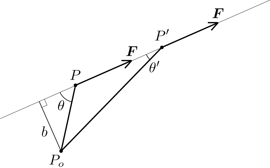
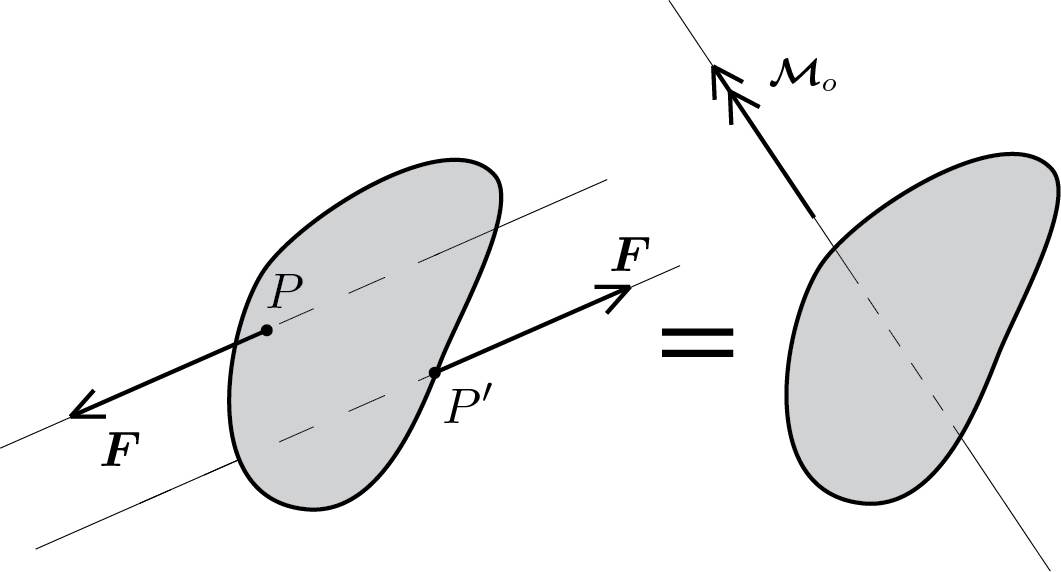
Given a force \(\vec{F} \) applied to point identified by vector \(\vec{X} \) and given a pole identified by \(\vec{X}_o \text{,}\) it is possible to evaluate the moment, or torque, of \(\vec{F}\) with respect to the chosen pole by calculating the following vector product

\begin{equation} \calvec{M}_o = \left( \vec{X} - \vec{X}_o\right) \times \vec{F}\,,\tag{5.1.9} \end{equation}

where \(\calvec{M}_o\) is a vector orthogonal to both vectors \(\left( \vec{X} - \vec{X}_o\right)\) and \(\vec{F}\) and its modulus is

\begin{equation} \|\calvec{M}_o\| = \|\left( \vec{X} - \vec{X}_o\right)\| \|\vec{F}\| \sin{\theta}\,,\tag{5.1.10} \end{equation}

being \(\theta\) the angle between the two vectors. The quantity

\begin{equation} b = \|\left( \vec{X} - \vec{X}_o\right)\| \sin{\theta}\tag{5.1.11} \end{equation}

takes the name of moment arm quantity that does not change if the force changes position along its line of application:

\begin{equation*} b = \|\left( \vec{X} - \vec{X}_o\right)\| \sin{\theta} = \|\left( \vec{X}' - \vec{X}_o\right)\| \sin{\theta'}\,. \end{equation*}

Then \(b\) is the distance between the pole \(P_o\) and the line of application of the force \(\vec{F}\text{.}\) It worth of notig that if \(\theta=0\) or \(\theta=\pi\text{,}\) i.e. vectors \(\left( \vec{X} - \vec{X}_o\right)\) and \(\vec{F}\) are parallel, the moment \(\calvec{M}_o\) is null.

🔗

Note 5.1.4. moment of a couple.

\begin{equation*} \| \calvec{M}_o \| = \|\vec{F}\|\, b \end{equation*}

\(b \)

🔗

Prev Top Next