Solid Mechanics - the continuity hypothesis

Section 2.1 the continuity hypothesis

At the basis of the continuum mechanics there is the idea of studying different physical phenomena without a precise knowledge of the internal micro-structure of the matter by adopting the so-called macroscopic point of view. In other words, all the used quantities represent an average of all the processes taking place at atomic or molecular scale.

The macroscopic systems thus defined can be effectively described using the continuous approach which assumes, for the body under examination, a continuous distribution of matter in space and time. The body is always seen as an assembly of single particles or points which have not to be confused with the point mass systems of Newtonian mechanics or the particle systems of atomic theory. Typically the point of a continuous body inside it hides an internal structure (an accumulation of molecules or atoms or an heterogeneous composition of various constituents) of sufficiently small dimensions if compared with the scale of the problem under consideration. The behavior of the point or particle is a consequence of the collective behavior of all that inside constitutes the point of the continuum.

The continuity hypothesis has important consequences.

The possibility of making a one-to-one association between the points of the body and the points of the Euclidean space region occupied by the body.
The possibility of dividing a body into smaller and smaller volume regions and of always finding the same physical characteristics as the volume decreases.
The analyticity of the functions used to describe the physical phenomenon under examination allows to formulate the fundamental laws of mechanics in terms of differential equations.
The macroscopic approach at the basis of continuum mechanics can be used in the study of solids, fluids and gases.

Subsection 2.1.1 geometric description of the bodies

The continuity hypothesis allows to identify the body with an open subset \(\body \) of the Euclidean space. As already discussed in the chapter dedicated to kinematics, the body will assume different configurations. In the following we will refer to a generic configuration assumed by the body during its motion. On this configuration it is possible to calculate, for example, the volume occupied by the body

\begin{equation} \func{v}{\body} = \int_{\body} dv \,.\tag{2.1.1} \end{equation}

Subsection 2.1.2 mass

Mass is a property of matter that quantifies its resistance to acceleration. According to the continuity hypothesis, the mass is assumed to be distributed continuously over the whole body. In particular we assume the existence of a scalar field \(\func {\rho} {\vec{x}}> 0 \) denoted mass density such that

\begin{equation} \func{m}{\body} = \int_{\body} \func{\rho}{\vec{x}} dv \,.\tag{2.1.2} \end{equation}

A formal definition of the mass can be made as follows. Let \(\vec{x} \) be a point in \(\body \) and let \(\func{\body_{\delta}}{\vec{x}}\) a family of volumes such that \(\func{v}{\func{\body_{\delta}}{\vec{x}}} \rightarrow 0 \) if \(\delta \rightarrow 0 \text{.}\) Then

\begin{equation} \func{\rho}{\vec{x}} = \lim_{\delta \to 0} \frac{\func{m}{\func{\body_{\delta}}{\vec{x}}}}{\func{v}{\func{\body_{\delta}}{\vec{x}}}} \,.\tag{2.1.3} \end{equation}

If this limit exists and is positive in every point \(\vec{x}\) of the body then the hypothesis of continuity is verified. In addition, the limit must always be the same for any volume family \(\func{\body_{\delta}} {\vec{x}} \) having the described property.

Note 2.1.2.

The modern idea of the limit of a function dates back to Bolzano which, in 1817, introduced the basics of the epsilon-delta technique to define continuous functions. However, his work was not known during his lifetime. The French mathematician Augustin-Louis Cauchy, in his book of the “Cours d'analyse” of 1821, discussed variable quantities, infinitesimals and limits and defined the continuity of \(y = f(x) \) establishing that a infinitesimal variation in \(x\) necessarily produces an infinitesimal variation in \(y \text{.}\)

Cauchy was the first to formulate continuum mechanics in the 19th century.

Subsection 2.1.3 forces

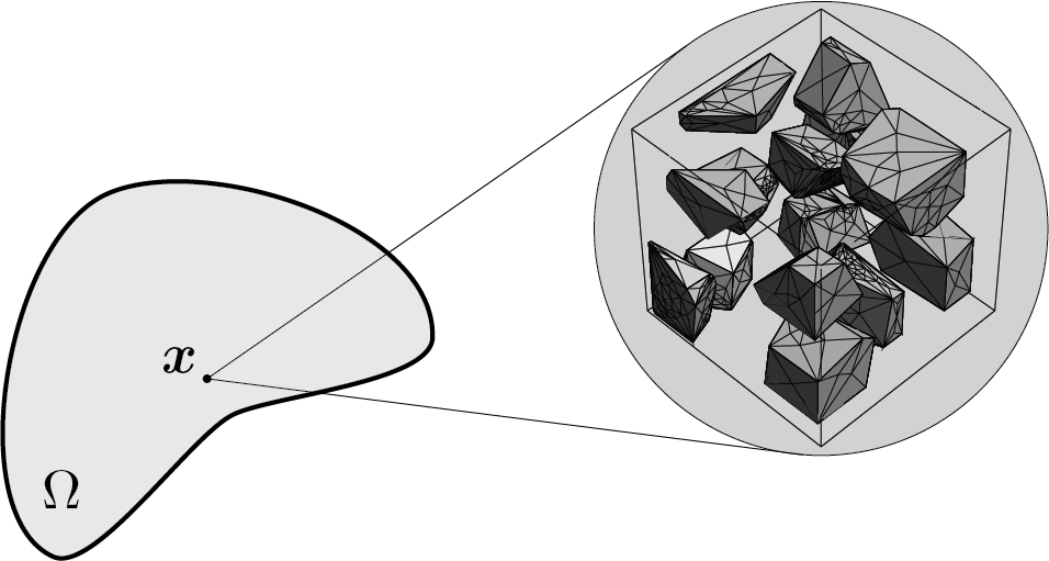
The mechanical interaction between parts of a body or body with the surrounding environment is described by means of forces. Two types of forces are considered: volume forces, which act within the body, and surface forces, which are exerted through a surface. For the hypothesis of continuity, as done for the mass, also the forces are postulated through the existence of vector fields that allow to calculate the resultant of all the forces acting on the body

\begin{equation} \func{\vec{R}}{\body} = \int_{\body} \vec{b} \, dv + \int_{\partial\body} \vec{t} \, ds \,,\label{body_resultant}\tag{2.1.4} \end{equation}

and the resultant torque, with respect to the origin, of the applied forces

\begin{equation} \func{\calvec{M}}{\body} = \int_{\body} \vec{x} \times \vec{b} \, dv + \int_{\partial\body} \vec{x} \times \vec{t} \, ds \,.\label{body_resultant_moment}\tag{2.1.5} \end{equation}

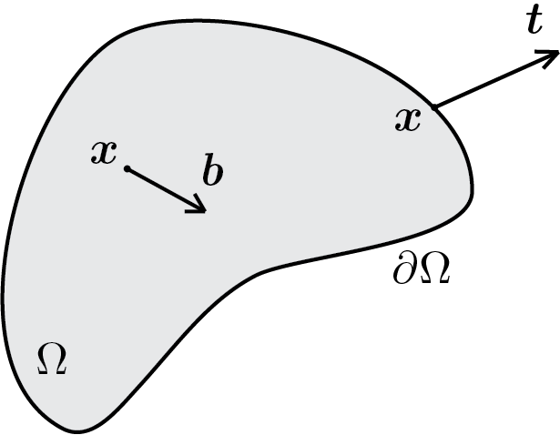
where \(\partial \body \) is the boundary of \(\body\) and therefore it is a surface, \(\vec{b} \) and \(\vec{t} \) denote two vector fields which will be better described below and which represent, respectively, a bulk force density or, simply, the bulk force and a surface force density that will be called traction.

Subsubsection 2.1.3.1 bulk force

A bulk force does not arise due to a physical contact between bodies but is the result of remote action, for example the gravitational force. We therefore assume the existence of a vector field \(\func{\vec{b}} {\vec{x}} \) depending on the position of the point \(\vec{x} \) belonging to \(\body \text{.}\) Similarly to what has been done for mass density, it is possible to give a formal definition of \(\func{\vec{b}} {\vec{x}} \text{:}\)

\begin{equation} \func{\vec{b}}{\vec{x}} = \lim_{\delta \to 0} \frac{\func{\vec{F}}{\func{\body_{\delta}}{\vec{x}}}}{\func{v}{\func{\body_{\delta}}{\vec{x}}}} \,,\tag{2.1.6} \end{equation}

where \(\func{\vec{F}}{\func{\body_{\delta}}{\vec{x}}}\) is the force acting on volume \(\func{\body_{\delta}}{\vec{x}}\text{.}\)

Subsubsection 2.1.3.2 traction

Traction comes from physical contact between bodies. Contact can take place through \(\partial \body \text{,}\) the boundary of the body, and in this case there will be an external traction. Or, as we will discuss more extensively in the following sections, it can take place through an ideal surface passing inside the body, in this case we will speak of an internal traction. We therefore introduce a formal definition of traction which will allow us to specify the dependence of this vector field.

Given a point \(\vec{x} \) of the body placed inside or on the border of \(\body \text{,}\) and given a family of surfaces \(\func{\Gamma_{\delta}} {\vec{x}} \) passing through this point such that \(\func{a} {\func{\Gamma_{\delta}} {\vec{x}}} = \int_{\Gamma_\delta} ds \rightarrow 0 \) if \(\delta \rightarrow 0 \text{,}\) we assume the existence of a vector field \(\func{\vec{t}} {\vec{x}, \Gamma_{\delta}} \) defined as follows

\begin{equation} \func{\vec{t}}{\vec{x},\Gamma_{\delta}} = \lim_{\delta \to 0} \frac{\func{\vec{F}}{\func{\Gamma_{\delta}}{\vec{x}}}}{\func{a}{\func{\Gamma_{\delta}}{\vec{x}}}} \,,\tag{2.1.7} \end{equation}

where \(\func{\vec{F}}{\func{\Gamma_{\delta}}{\vec{x}}}\) is a surface force acting on the area \(\func{\Gamma_{\delta}}{\vec{x}}\text{.}\) \(\func{\vec{t}}{\vec{x}, \Gamma_{\delta}}\) is called traction vector, or simply traction, depending on the position \(\vec{x}\) and on the family of surfaces passing through \(\vec{x}\text{.}\)

A suitable definition of this dependence, elaborated by Cauchy, leads to the notion of Cauchy stress tensor.