Solid Mechanics - Cauchy stress tensor tensor

Section 2.3 Cauchy stress tensor tensor

Subsection 2.3.1 Cauchy's postulate

In previous sections, the traction \(\func{\vec{t}}{\vec{x}, \Gamma_{\delta}} \) was formulated with a very generic dependence on the surface \(\Gamma_{\delta}\) passing through the point \(\vec{x}\text{.}\) On the basis of Cauchy's postulate, fundamental for all subsequent developments, it is assumed instead

\begin{equation} \func{\vec{t}}{\vec{x},\Gamma_{\delta}} = \func{\vec{t}}{\vec{x},\vec{n}}\,,\tag{2.3.1} \end{equation}

where \(\vec{n}\) represents the normal direction to the surface identified by a vector of unit length. Therefore the absolute independence of the traction vector from other factors, such as the curvature of the surface passing through the point \(\vec{x}\text{,}\) is postulated. The figure below shows some surfaces passing through the point \(\vec{x}\) and sharing in this point the very same tangent to the surface and therefore the same normal direction.

Subsection 2.3.2 Cauchy stress Theorem

A series of results are presented which, taken together, constitute the Cauchy stress tensor Theorem, the statement of which will be given at the end of the section.

Subsubsection 2.3.2.1 equilibrium of Cauchy's tetrahedron

The application of Eq. (2.2.3) assuming as subdomain \(\omega\) the Cauchy tetrahedron illustrated in the previous video provides

\begin{equation*} \int_{\omega_{\delta}} \func{\vec{b}}{\vec{x}} \, dv + \int_{\partial\omega_{\delta}} \func{\vec{t}}{\vec{x}, \vec{n}} \, ds = \vec0\,. \end{equation*}

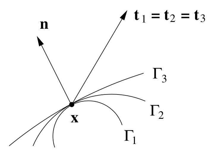
It has already been observed that when \(\delta \to 0 \) the volume measurement \(\omega_{\delta} \) tends to zero much faster than the surface measurement \(\partial\omega_{\delta}\text{.}\) Moreover \(\partial\omega_{\delta} = \Gamma_{\delta}\cup\Gamma_{1}\cup\Gamma_{2}\cup\Gamma_{3}\text{,}\) then previous equation becomes

\begin{equation*} \int_{\Gamma_{\delta}} \func{\vec{t}}{\vec{x}, \vec{n}} \, ds + \int_{\Gamma_{1}} \func{\vec{t}}{\vec{x}, -\vec{e}_1} \, ds + \int_{\Gamma_{2}} \func{\vec{t}}{\vec{x}, -\vec{e}_2} \, ds + \int_{\Gamma_{3}} \func{\vec{t}}{\vec{x}, -\vec{e}_3} \, ds = \vec0\,. \end{equation*}

Taking into account the geometric relationship of face \(\Gamma_{\delta}\) with each face \(\Gamma_{1}\text{,}\) \(\Gamma_{2}\) and \(\Gamma_{3}\text{,}\) it can be obtained what follows

\begin{equation*} \func{\vec{t}}{\vec{x}, \vec{n}}\,\Gamma_{\delta} + \func{\vec{t}}{\vec{x}, -\vec{e}_1} \,\Gamma_{\delta}\,n_1 + \func{\vec{t}}{\vec{x}, -\vec{e}_2} \,\Gamma_{\delta}\,n_2 + \func{\vec{t}}{\vec{x}, -\vec{e}_3} \,\Gamma_{\delta}\,n_3 = \vec0\,, \end{equation*}

and finally

\begin{equation} \func{\vec{t}}{\vec{x}, \vec{n}} = - \func{\vec{t}}{\vec{x}, -\vec{e}_1} \,n_1 - \func{\vec{t}}{\vec{x}, -\vec{e}_2} \,n_2 - \func{\vec{t}}{\vec{x}, -\vec{e}_3} \,n_3 \,.\label{cauchy_tetrahedron_eq}\tag{2.3.2} \end{equation}

Subsubsection 2.3.2.2 principle of action and reaction

If in Eq. (2.3.2) \(\vec{n}=\vec{e}_1\) is assumed, the following raltionship is obtained

\begin{equation} \func{\vec{t}}{\vec{x}, \vec{e_1}} = - \func{\vec{t}}{\vec{x}, -\vec{e}_1} \,.\label{cauchy_action_reaction_eq}\tag{2.3.3} \end{equation}

The very same condition is true for \(\vec{n}=\vec{e}_2\) and \(\vec{n}=\vec{e}_3\text{.}\)

Subsubsection 2.3.2.3 the tensor

By using Eqs. (2.3.2) and (2.3.3) the following result is obtained

\begin{equation} \func{\vec{t}}{\vec{x}, \vec{n}} =\func{\vec{t}}{\vec{x}, \vec{e}_1} \,n_1 + \func{\vec{t}}{\vec{x}, \vec{e}_2} \,n_2 + \func{\vec{t}}{\vec{x}, \vec{e}_3} \,n_3 \,,\label{cauchy_lt_eq}\tag{2.3.4} \end{equation}

relationship showing how traction \(\vec{t}\) is linked to the generic normal \(\vec{n}\) by means of a linear transformation, see video on linear transformations in Section 1.2, represented by a second order tensor. Then

\begin{equation} \func{\vec{t}}{\vec{x}, \vec{n}} =\func{\tens{\sigma}}{\vec{x}}\,\vec{n} \,.\label{cauchy_stress_eq}\tag{2.3.5} \end{equation}

\(\func{\tens{\sigma}}{\vec{x}}\) prende il nome di tensore della tensione di Cauchy.

The matrix form of previous relationship is

\begin{equation} \left[\begin{array}{c}t_1\\t_2\\t_3\end{array}\right] = \left[\begin{array}{ccc} \sigma_{11} \amp \sigma_{12} \amp \sigma_{13} \\ \sigma_{21} \amp \sigma_{22} \amp \sigma_{23} \\ \sigma_{31} \amp \sigma_{32} \amp \sigma_{33} \end{array}\right] \left[\begin{array}{c}n_1\\n_2\\n_3\end{array}\right]\,,\label{cauchy_mat_stress_eq}\tag{2.3.6} \end{equation}

where the 9 components of the stress tensor appear explicitly. These components can be visulized as follows,

i.e. each column of the matrix associated to the stress tensor,

\begin{equation} \mat{\sigma} = \left[\begin{array}{ccc}\vec{t}_{\vec{e}_1} \amp \vec{t}_{\vec{e}_2} \amp \vec{t}_{\vec{e}_3}\end{array}\right]\,,\tag{2.3.7} \end{equation}

collects the components of one of the three tractions relative to the planes identified by coordinate axes.

Subsubsection 2.3.2.4 differential form of equilibrium equations

Consider the cancellation condition of the resultant of the applied forces, equation (2.2.3). This equation, thanks to the (2.3.5), can be reformulated as follows

\begin{equation*} \int_{\omega} \vec{b} \, dv + \int_{\partial\omega} \tens{\sigma}\,\vec{n} \, ds = \vec0\,. \end{equation*}

By the divergence theorem the surface integral can be transformed thus obtaining

\begin{equation*} \int_{\omega} \left( \text{div}\tens{\sigma} + \vec{b} \right) \, dv = \vec0\,. \end{equation*}

For the continuity hypothesis, this equation must be satisfied for any subdomain \(\omega \) of the body under examination, therefore the following differential equation is obtained

\begin{equation} \text{div}\tens{\sigma} + \vec{b} = \vec0\tag{2.3.8} \end{equation}

to be satisfied in every point of the body \(\body \text{.}\) This vector equation is called indefinite equation of equilibrium or, referring to the three scalar equations relative to the vector components, indefinite equations of equilibrium.

Subsubsection 2.3.2.5 symmetry of the tensor

The equilibrium condition regarding the resultant torque, equation (2.2.4), allows to establish the symmetry of the stress tensor. However, its explicit derivation is not presented here. The interested reader can find more details in the reference given at the end of the chapter.

Theorem 2.3.3 (A.-L. Cauchy).

Given a body subject to some applied loads, a necessary and sufficient condition for the body to be in equilibrium (satisfaction of Eqs. (2.2.1) and (2.2.2)) is that there is a tensor field \(\func{\tens{\sigma}}{\vec{x}} \) such that

\begin{equation} \func{\vec{t}}{\vec{x}, \vec{n}} =\func{\tens{\sigma}}{\vec{x}}\,\vec{n}\,,\label{T_cauchy_stress_eq}\tag{2.3.9} \end{equation}

\begin{equation} \text{div}\tens{\sigma} + \vec{b} = \vec0\,,\label{T_cauchy_equilibrium_eq}\tag{2.3.10} \end{equation}

\begin{equation} \transp{\tens{\sigma}}=\tens{\sigma}\,.\label{T_cauchy_simmetry_eq}\tag{2.3.11} \end{equation}

Remark 2.3.4. observations about indefinite equations of equilibrium.

The equations (2.3.10) do not completely determine the Cauchy stress tensor field for a body in equilibrium. In particular, there are 3 differential equations to calculate, for the symmetry of the tensor, the \(6\) unknown components of \(\tens{\sigma} \text{.}\) As will be seen in the following, this drawback will be solved by characterizing the constitutive behavior of the material of which the body is composed. Behavior to be reconstructed experimentally and referring to the average of the quantities involved. Remember that the macroscopic approach is not based on a precise description of the internal micro-structure of matter.
The boundary conditions to be associated with the differential equations (2.3.10) will be determined by relating the unknown stress \(\tens{\sigma} \) to the tractions, \(\bar {\vec{t}} \text{,}\) assigned on the contour of the body \(\body \text{.}\) This relationship is established through the (2.3.9) which provides
\begin{equation} \tens{\sigma}\,\vec{n} = \bar{\vec{t}}\,, \text{su}\;\partial\body\,.\tag{2.3.12} \end{equation}
These equations constitute the boundary conditions of the natural type for the differential problem (2.3.10).
At the basis of the derivation of the equations (2.3.10) there is the hypothesis of continuity of the vector field \(\vec{b} \) and the hypothesis of differentiability of the tensor field \(\tens{\sigma} \text{.}\) Hypotheses that allow, as seen, to pass from equations in integral form to equations in local form.