
Section 1.7 stretch tensor \(\tens{U}\) and principal directions (transformation of line elements)

The identification of the prinicipal directions of the stretch tensor allows to obtain an “intrinsic” representation of the deformation to which a generic point of the body is subjected. The adjective “intrinsec” is justified because, as we will see, a simpler representation of the deformation state is obtained but, above all, independent of the reference system used.

The discussion that follows, gradually, presents the idea behind the principal directions referring to the right stretch tensor, \(\tens{U}\text{,}\) in a particular form: the diagonal form.

With due clarifications, what is obtained also applies to the left stretch tensor, \(\tens{V}\text{.}\)

Subsection 1.7.1

Let us assume for \(\tens{U}\) the following diagonal form

\begin{equation} \mat{U} = \left[\begin{array}{ccc} \lambda \amp 0 \amp 0\\ 0 \amp \lambda \amp 0\\ 0 \amp 0 \amp \lambda\\ \end{array}\right]\,.\tag{1.7.1} \end{equation}

If \(\tens{U}\) is applied to a generic vector \(\vec{v}\) the following result is obtained

\begin{equation} \mat{U}\mat{v} = \left[\begin{array}{ccc} \lambda \amp 0 \amp 0\\ 0 \amp \lambda \amp 0\\ 0 \amp 0 \amp \lambda\\ \end{array}\right] \left[\begin{array}{c}v_1\\v_2\\v_3\end{array}\right] = \lambda \left[\begin{array}{ccc} 1 \amp 0 \amp 0\\ 0 \amp 1 \amp 0\\ 0 \amp 0 \amp 1\\ \end{array}\right] \left[\begin{array}{c}v_1\\v_2\\v_3\end{array}\right] = \lambda \mat{I} \mat{v} = \lambda \mat{v} \,.\tag{1.7.2} \end{equation}

Result that shows how in this case the application of \(\tens{U}\) to any vector determines only a scaling, proportional to the factor \(\lambda\text{,}\) of the length of the vector which maintains the original direction. It is easy to verify that

\begin{equation*} \|\tens{U}\vec{v} \| = \|\lambda\vec{v} \| = |\lambda| \|\vec{v} \|\,. \end{equation*}

Moreover because

\begin{equation*} \det{\tens{F}} = \det{\tens{R}\tens{U}} = \det{\tens{U}} = \lambda^3 > 0 \end{equation*}

the unique admissible value for \(\lambda\) is

\begin{equation*} \lambda > 0\,. \end{equation*}

We can summarize what has been achieved as follows. Each direction is a principal direction since the transformed vectors maintain the original direction. The scaling factor \(\lambda\text{,}\) which is called principal stretch, applies to any direction on which \(\tens{U}\) is applied by determining one of the following effects

  • \(\lambda > 1\text{,}\) the vector increases its length;
  • \(\lambda = 1\text{,}\) the vector does not modify its length;
  • \(\lambda < 1\text{,}\) the vector decreases its length;
  • \(\lambda = 0\text{,}\) the value is not admissible because the resulting vector cannot go to zero length;
  • \(\lambda < 0\text{,}\) the value is not admissible because the resulting vector cannot point in the opposite direction.

Subsection 1.7.2

Now suppose for \(\tens{U}\) always a diagonal form but with coefficients not all equal to each other. In particular, let us take

\begin{equation} \mat{U} = \left[\begin{array}{ccc} \lambda_1 \amp 0 \amp 0\\ 0 \amp \lambda_1 \amp 0\\ 0 \amp 0 \amp \lambda_2\\ \end{array}\right]\,.\tag{1.7.3} \end{equation}

By applying \(\tens{U}\) to the following vectors

\begin{equation*} \mat{u} = \left[\begin{array}{c}u_1\\u_2\\0\end{array}\right] \,,\quad \mat{v} = \left[\begin{array}{c}0\\0\\v_3\end{array}\right] \,,\quad \mat{w} = \left[\begin{array}{c}w_1\\w_2\\w_3\end{array}\right] \,, \end{equation*}

we obtain

\begin{equation*} \mat{U}\mat{u} = \lambda_1\mat{u} \,,\quad \mat{U}\mat{v} = \lambda_2\mat{v} \,,\quad \mat{U}\mat{w} = \left[\begin{array}{c}\lambda_1\,w_1\\\lambda_1\,w_2\\\lambda_2\,w_3\end{array}\right] \,.\quad \end{equation*}

Result that can be commented as follows.

  • All the vectors belonging to directions lying in the plane identified by the first two reference axes are simply scaled by the factor \(\lambda_1\text{.}\)
  • Vectors parallel to the third reference axis are simply scaled by the factor \(\lambda_2\text{.}\)
  • All other vectors are both scaled and change direction and the scale factor depends on both \(\lambda_1 \) and \(\lambda_2 \text{.}\)

Then in this case principal directions are given by all the directions belonging to the \(1-2\) plane and by the \(3\) axis.

As for the scaling factors \(\lambda_1 \) and \(\lambda_2 \) it can be observed as in the previous case as

\begin{equation*} \det{\tens{F}} = \det{\tens{R}\tens{U}} = \det{\tens{U}} = \lambda_1^2\,\lambda_2 > 0 \end{equation*}

condition which allows to state

\begin{equation*} \lambda_2 > 0\,. \end{equation*}

While the positivity condition of the tensor \(\tens{U} \)

\begin{equation*} \vec{u} \cdot \tens{U} \vec{u} = \vec{u} \cdot \lambda_1 \vec{u} = \lambda_1\,\vec{u} \cdot \vec{u} > 0\,,\quad \forall \vec{u} \neq \vec0\,, \end{equation*}

gives also

\begin{equation*} \lambda_1 > 0\,. \end{equation*}

Therefore also in this case \(\lambda_1 \) and \(\lambda_2 \) assume the meaning of scale factors called principal stretches of the line elements belonging to the principal directions. For \(\lambda_1 \) and \(\lambda_2 \) the same considerations discussed in the previous case apply.

All the considerations made so far apply if the tensor \(\tens{U} \) takes the form

\begin{equation*} \mat{U} = \left[\begin{array}{ccc} \lambda_1 \amp 0 \amp 0\\ 0 \amp \lambda_2 \amp 0\\ 0 \amp 0 \amp \lambda_1\\ \end{array}\right] \,, \end{equation*}

with principal directions defined by the \(1-3\) plane and the \(2\) axis; or the form

\begin{equation*} \mat{U} = \left[\begin{array}{ccc} \lambda_2 \amp 0 \amp 0\\ 0 \amp \lambda_1 \amp 0\\ 0 \amp 0 \amp \lambda_1\\ \end{array}\right] \,, \end{equation*}

with principal directions defined by the \(2-3\) plane and the \(1\) axis.

Subsection 1.7.3

It is now clear that the more generic diagonal form of the tensor \(\tens{U} \) is given by

\begin{equation} \mat{U} = \left[\begin{array}{ccc} \lambda_1 \amp 0 \amp 0\\ 0 \amp \lambda_2 \amp 0\\ 0 \amp 0 \amp \lambda_3\\ \end{array}\right]\,,\label{diag_U_eq}\tag{1.7.4} \end{equation}

where all the coefficients on the main diagonal are generally different. In this case, avoiding repeating further considerations now obvious, the following results can be established.

  • Only \(\vec{e}_{1}\text{,}\) \(\vec{e}_{2}\) and \(\vec{e}_{3}\) axes constitute the principal directions of tensor \(\tens{U}\text{.}\)
  • The principal stretches, \(\lambda_{1}\text{,}\) \(\lambda_{2}\) and \(\lambda_{3}\text{,}\) are positive real numbers associated to \(\vec{e}_{1}\text{,}\) \(\vec{e}_{2}\) and \(\vec{e}_{3}\text{,}\) respectively. Under the action of the transformation, line elements belonging to principal directions maintain the original direction by changing only their length that can increase or decrease.

Subsection 1.7.4 spectral decomposition of the stretch tensor

The diagonal form of \(\tens{U}\text{,}\) see (1.7.4), can be written as follows

\begin{equation*} \mat{U} = \lambda_1 \left[\begin{array}{ccc} 1 \amp 0 \amp 0\\ 0 \amp 0 \amp 0\\ 0 \amp 0 \amp 0 \end{array}\right] + \lambda_2 \left[\begin{array}{ccc} 0 \amp 0 \amp 0\\ 0 \amp 1 \amp 0\\ 0 \amp 0 \amp 0 \end{array}\right] + \lambda_3 \left[\begin{array}{ccc} 0 \amp 0 \amp 0\\ 0 \amp 0 \amp 0\\ 0 \amp 0 \amp 1 \end{array}\right] \,, \end{equation*}

from which, on the basis of the discussion presented in the previous video, the following expression for \(\tens{U}\) can be obtained

\begin{equation} \tens{U} = \lambda_1\,\vec{e}_1 \otimes \vec{e}_1 + \lambda_2\,\vec{e}_2 \otimes \vec{e}_2 + \lambda_3\,\vec{e}_3 \otimes \vec{e}_3\,.\tag{1.7.5} \end{equation}

The latter result is of fundamental importance because it allows you to express \(\tens{U}\) with respect to the principal directions in the more general, and also more frequent, case of principal directions not aligned with the axes of reference used in the problem under consideration.

Let the generic principal directions be noted by \(\vec{u}_{1}\text{,}\) \(\vec{u}_{2}\) and \(\vec{u}_{3}\text{,}\) then the spectral decomposition of tensor \(\tens{U}\) is

\begin{equation} \tens{U} = \lambda_1\,\vec{u}_{1} \otimes \vec{u}_{1} + \lambda_2\,\vec{u}_{2} \otimes \vec{u}_{2} + \lambda_3\,\vec{u}_{3} \otimes \vec{u}_{3}\,.\label{spectral_U_eq}\tag{1.7.6} \end{equation}

The principal stretches constitute what is called the spectrum of \(\tens{U}\text{.}\)

Remark 1.7.1.

Ever since we started talking about principal directions, we never mentioned the symmetry of \(\tens{U}\text{.}\) The symmetry of the tensor determines the mutual orthogonality of the principal directions, whatever direction they take.

Remark 1.7.2.

The spectral form (1.7.6) explains why, compared to the standard reference base, the matrix associated to tensor \(\tens{U}\) almost always loses its diagonal form. In fact, although the principal directions are always present, these in general do not coincide with the axes of the standard reference system. The loss of the diagonal form can be highlighted by a matrix writing of the spectral decomposition of the tensor

\begin{equation} \mat{U} = \begin{array}{l} \lambda_1 \left[\begin{array}{ccc} u_{11}u_{11} \amp u_{11}u_{21} \amp u_{11}u_{31}\\ u_{21}u_{11} \amp u_{21}u_{21} \amp u_{21}u_{31}\\ u_{31}u_{11} \amp u_{31}u_{21} \amp u_{31}u_{31} \end{array}\right] +\\ \lambda_2 \left[\begin{array}{ccc} u_{12}u_{12} \amp u_{12}u_{22} \amp u_{12}u_{32}\\ u_{22}u_{12} \amp u_{22}u_{22} \amp u_{22}u_{32}\\ u_{32}u_{12} \amp u_{32}u_{22} \amp u_{32}u_{32} \end{array}\right] +\\ \lambda_3 \left[\begin{array}{ccc} u_{13}u_{13} \amp u_{13}u_{23} \amp u_{13}u_{33}\\ u_{23}u_{13} \amp u_{23}u_{23} \amp u_{23}u_{33}\\ u_{33}u_{13} \amp u_{33}u_{23} \amp u_{33}u_{33} \end{array}\right]\,. \end{array}\label{mat_spectral_U_eq}\tag{1.7.7} \end{equation}

Where the following notation has been adopted for the components of the prinicipal directions

\begin{equation*} \mat{u_1} = \left[\begin{array}{c}u_{11}\\u_{21}\\u_{31}\end{array}\right] \,,\quad \mat{u_2} = \left[\begin{array}{c}u_{12}\\u_{22}\\u_{32}\end{array}\right] \,,\quad \mat{u_3} = \left[\begin{array}{c}u_{13}\\u_{23}\\u_{33}\end{array}\right] \,. \end{equation*}

Finally it is interesting to observe how the expression (1.7.7) can be written in the following way

\begin{equation*} \mat{U} = \left[\begin{array}{ccc} u_{11} \amp u_{12} \amp u_{13}\\ u_{21} \amp u_{22} \amp u_{23}\\ u_{31} \amp u_{32} \amp u_{33} \end{array}\right] \left[\begin{array}{ccc} \lambda_1 \amp 0 \amp 0\\ 0 \amp \lambda_2 \amp 0\\ 0 \amp 0 \amp \lambda_3\\ \end{array}\right] \transp{ \left[\begin{array}{ccc} u_{11} \amp u_{12} \amp u_{13}\\ u_{21} \amp u_{22} \amp u_{23}\\ u_{31} \amp u_{32} \amp u_{33} \end{array}\right] }\,, \end{equation*}

which is how the expression assumed by the tensor \(\tens{U} \) is evaluated when passing from the coordinate system consisting of the principal directions to the standard coordinate system \(\vec{e}_1 \text{,}\) \(\vec{e}_2 \) and \(\vec{e}_3 \text{.}\) The matrix used for the transformation is constructed by inserting in the columns the vectors \(\vec{u}_{1} \text{,}\) \(\vec{u}_{2} \) and \(\vec{u}_{3}\text{.}\)

Let \(\tens{U}\) be given by the following diagonal form

\begin{equation*} \mat{U} = \left[\begin{array}{ccc} 2 \amp 0 \amp 0\\ 0 \amp 5 \amp 0\\ 0 \amp 0 \amp 7\\ \end{array}\right]\,, \end{equation*}

calculate the expression assumed \(\tens{U}\) assuming to apply to the principal directions the following rotations

\begin{equation*} \matWp{R}{1} = \left[\begin{array}{ccc} \cos{\frac{\pi}{4}} \amp -\sin{\frac{\pi}{4}} \amp 0\\ \sin{\frac{\pi}{4}} \amp \cos{\frac{\pi}{4}} \amp 0\\ 0 \amp 0 \amp 1\\ \end{array}\right]\,, \end{equation*}
\begin{equation*} \matWp{R}{2} = \left[\begin{array}{ccc} \cos{\frac{\pi}{4}} \amp 0 \amp -\sin{\frac{\pi}{4}}\\ 0 \amp 1 \amp 0\\ \sin{\frac{\pi}{4}} \amp 0 \amp \cos{\frac{\pi}{4}}\\ \end{array}\right]\,. \end{equation*}

The following MATLAB® instructions allow you to calculate what is required.

R1 = [cos(pi/4) -sin(pi/4) 0; sin(pi/4) cos(pi/4) 0; 0 0 1];
R2 = [cos(pi/4) 0 -sin(pi/4); 0 1 0; sin(pi/4) 0 cos(pi/4)];
u1 = R2*R1*[1; 0; 0];
u2 = R2*R1*[0; 1; 0];
u3 = R2*R1*[0; 0; 1];
lam1 = 2;
lam2 = 5;
lam3 = 7;
U = lam1*u1*transpose(u1) + lam2*u2*transpose(u2) + ...
lam3*u3*transpose(u3)
Listing 1.7.3.

Also carry out the following calculation.

u1*transpose(u1) + u2*transpose(u2) + u3*transpose(u3)
Listing 1.7.4.
What does the obtained result suggest?

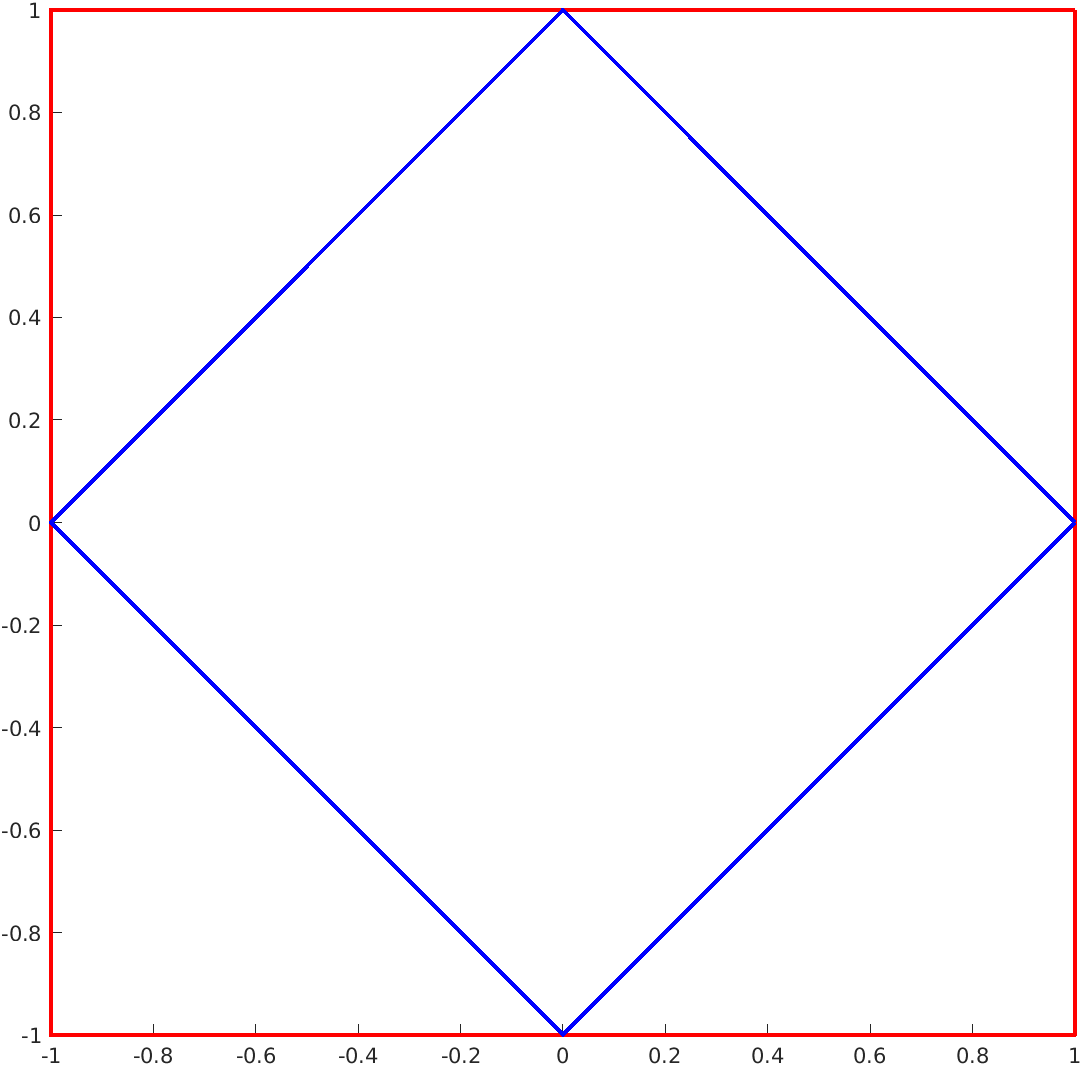
In order to verify how the tensor \(\tens{U}\) acts differently on the principal directions and on the directions identified by the standard reference, consider the following plane state characterized by the following diagonal form of \(\tens{U} \)

\begin{equation*} \mat{U} = \left[\begin{array}{cc} 1.2\lambda \amp 0\\ 0 \amp \lambda \end{array}\right]\,. \end{equation*}

Assume for the principal directions an inclination equal to \(\pi/4\) and then apply the stretch tensor to the two squares, represented in the following figure. The red square has sides aligned with the standard reference, the blue square has sides aligned with the principal directions.

Figure 1.7.5.

The application of the tensor is carried out by varying the parameter \(\lambda \text{,}\) from which the two eigenvalues of the tensor depend, between the values \(1.1\) and \(1.5\text{.}\)

The MATLAB® instructions that can be used for calculating and displaying the deformations of the two squares starting from the initial configurations are shown below.

Q1 = [1 -1 -1 1 1; 1 1 -1 -1 1];
Q2 = [1 0 -1 0 1; 0 1 0 -1 0];

x = Q1(1,:);
y = Q1(2,:);

pbaspect([1 1 1])
line(x,y,'Color','red','LineWidth',2)

x = Q2(1,:);
y = Q2(2,:);
line(x,y,'Color','blue','LineWidth',2)


u1 = [1/sqrt(2); 1/sqrt(2)];
u2 = [-1/sqrt(2); 1/sqrt(2)];
syms U(lam) 
U(lam) = [u1 u2]*diag([1.2*lam lam])*transpose([u1 u2]);


for v = 1.1:0.1:1.5
  UQ1 = U(v)*Q1;
  x = UQ1(1,:);
  y = UQ1(2,:);
  line(x,y,'Color','red','LineWidth',2)

  UQ2 = U(v)*Q2;
  x = UQ2(1,:);
  y = UQ2(2,:);
  line(x,y,'Color','blue','LineWidth',2)
end
Listing 1.7.6.

Subsection 1.7.5 eigenvalues and eigenvectors

Knowing the principal stretches \(\lambda_i\) and the principal directions, \(\vec{u}_i\) (\(i=1 \dots 3\)), associated with them, the spectral decomposition (1.7.6) allows to easily evaluate the tensor \(\tens{U} \) with respect to the reference system used.

The typical scenario is, however, reversed. That is, given the tensor \(\tens{U} \text{,}\) we want to evaluate the principal stretches and directions. Solving this question means calculating the eigenvalues and eigenvectors of the matrix associated with the tensor \(\tens{U}\text{.}\) In this section the procedure to be used in the solution of the eigenvalue problem will not be presented because this constitutes a topic that has certainly already been studied in previous courses and for which the available literature, also online, is vast. Here it was considered more important to highlight the mechanical meaning of eigenvalues and eigenvectors, meaning widely discussed in the previous sections.

In addition, MATLAB® will be used to calculate the eigenvalues and eigenvectors as shown in the following example.

Let us consider the expression of \(\tens{U}\) obtained in previous example, i.e.

\begin{equation*} \mat{U} = \left[\begin{array}{ccc} 5.2500 \amp -1.0607 \amp -1.7500 \\ -1.0607 \amp 3.5000 \amp -1.0607 \\ -1.7500 \amp -1.0607 \amp 5.2500 \end{array}\right]\,, \end{equation*}

calculate eigenvalues and eigenvectors by using MATLAB®. The required instructions are as follows.

U = ...
[5.2500 -1.0607 -1.7500; ...
-1.0607 3.5000 -1.0607; ...
-1.7500 -1.0607 5.2500];
[V, D] = eig(U)
Listing 1.7.7.

Insight 1.7.8. the characteristic polynomial.

The evaluation of the eigenvalues and eigenvectors associated with the tensor \(\tens{U}\) passes through the solution of the following cubic equation

\begin{equation*} -\lambda^3 + \func{I_1}{\tens{U}} \lambda^2 - \func{I_2}{\tens{U}} \lambda + \func{I_3}{\tens{U}} = 0\,, \end{equation*}

where the characteristic polynomial appears. It depends on three quantities that are called invariants of the tensor \(\tens{U} \text{.}\) The term invariant indicates that these values do not change as the reference system, with respect to which \(\tens{U}\) is represented, changes. In the following the expressions to be used for the calculation of the invariants are reported for the case regarding the tensor \(\tens{U} \) expressed with respect to the principal directions and for the generic case.

  • First invariant
    \begin{equation} \func{I_1}{\tens{U}} = \lambda_1 + \lambda_2 + \lambda_3 = \trace{\tens{U}}\,,\tag{1.7.8} \end{equation}
    where the trace of the tensor, i.e. the sum of the coefficients belonging to the main diagonal, is used.
  • Second invariant
    \begin{equation} \func{I_2}{\tens{U}} = \lambda_1\, \lambda_2 + \lambda_2\, \lambda_3 + \lambda_3\, \lambda_1 = \frac{1}{2}\left[(\trace{\tens{U}})^2 - \trace{\tens{U}^2}\right]\,.\tag{1.7.9} \end{equation}
  • Third invariant
    \begin{equation} \func{I_3}{\tens{U}} = \lambda_1\, \lambda_2\, \lambda_3 = \det{\tens{U}}\,.\tag{1.7.10} \end{equation}

Let us check that invariants do not change if we consider for \(\tens{U}\) its diagonal form

\begin{equation*} \mat{U} = \left[\begin{array}{ccc} 2 \amp 0 \amp 0\\ 0 \amp 5 \amp 0\\ 0 \amp 0 \amp 7\\ \end{array}\right]\,, \end{equation*}

or

\begin{equation*} \mat{U} = \left[\begin{array}{ccc} 5.2500 \amp -1.0607 \amp -1.7500 \\ -1.0607 \amp 3.5000 \amp -1.0607 \\ -1.7500 \amp -1.0607 \amp 5.2500 \end{array}\right]\,. \end{equation*}

MATLAB® instructions that can be used for the required check are reported here.

lam1 = 2;
lam2 = 5;
lam3 = 7;
I1 = lam1 + lam2 + lam3
I2 = lam1*lam2 + lam2*lam3 + lam3*lam1
I3 = lam1*lam2*lam3
U = ...
[5.2500 -1.0607 -1.7500; ...
-1.0607 3.5000 -1.0607; ...
-1.7500 -1.0607 5.2500];
I1 = trace(U)
I2 = 1/2*(trace(U)^2 - trace(U*U))
I3 = det(U)
Listing 1.7.9.