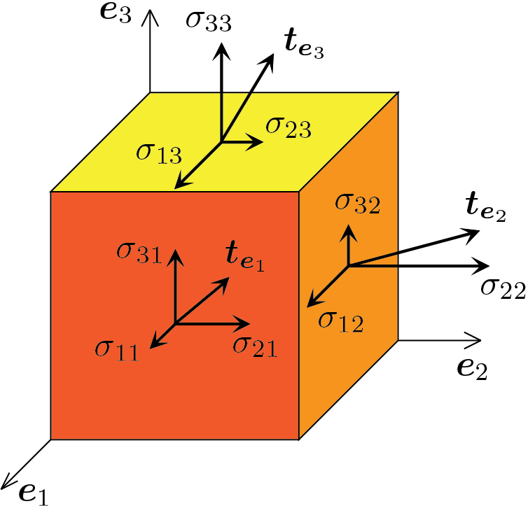
where the three reference planes are shown, i.e. the planes having the axes \(\vec{e}_1\text{,}\)\(\vec{e}_2\) and \(\vec{e}_3\) as outgoing normal. The components of the stress tensor refer to these planes, which are considered positive, and the figure shows these components according to the directions that are assumed to be positive. If we imagine of observing a cube, as the figure suggests, the hidden faces of the cube have the opposite directions \(-\vec{e}_1 \text{,}\)\(-\vec{e}_2 \) and \(-\vec{e}_3 \) as positive outgoing normal. On these planes, which are considered negative, the same stress components but of opposite sign will act. For example, the traction \(\vec{t}_{-\vec{e}_1} = -\vec{t}_{\vec{e}_1}\) will act on the plane having \(-\vec{e}_1 \) as normal.
which represents, see also the figure, the normal componente of traction \(\vec{t}_{\vec{e}_1}\text{.}\) By calculating the scalar product between \(\vec{t}_{\vec{e}_1}\) and direction \(\vec{e}_2\)
Similar assessments can be made for the other tractions \(\vec{t}_{\vec{e}_2}\) and \(\vec{t}_{\vec{e}_3}\text{.}\) A summary of the meaning of the components of the stress tensor is as follows.
are the normal components of the stress tensor. If the sign is positive they are traction components, if it is negative they are compression components.
constitute the tangential components of the tensor. The sign of the tangential components follows the convention indicated in the figure but, unlike the normal components, it has no particular physical meaning since the type of load does not change when the sign changes.
For each component of the tensor the second index refers to the plane’s normal on which the traction acts and the first index refers to the component of the traction.
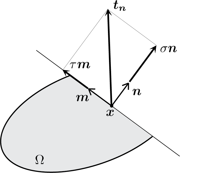
What has been discussed for the tensor components also applies to a generic normal \(\vec{n} \text{.}\) As established by the Cauchy tension theorem we have
To denote the two components, the convention, often adopted in the engineering field, which indicates the normal and tangential components with the symbols \(\sigma \) and \(\tau \) respectively, was used. The vector \(\vec{m} \text{,}\) like \(\vec{n} \text{,}\) is a vector of unit length.
Subsection2.4.2principal stresses and principal directions
What is discussed in Section 1.7 concerning the main directions of the tensor \(\tens{U} \) is also largely applicable to the stress tensor \(\tens{\sigma} \text{.}\) Both tensors are symmetric and the only fundamental distinction that needs to be made is that, unlike \(\tens{U} \text{,}\)\(\tens{\sigma} \) is not defined positive . Therefore in this case the eigenvalues, which now identify the principal stress of the tensor, can also be zero or negative. However the symmetry of \(\tens{\sigma} \) allows the writing of the spectral decomposition of the tensor
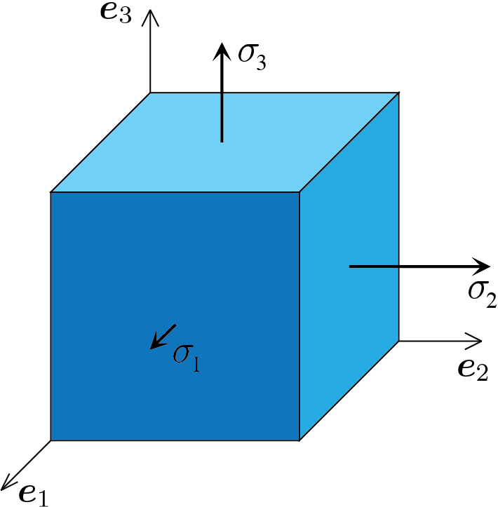
where the principal directions\(\vec{s}_1\text{,}\)\(\vec{s}_2\text{,}\)\(\vec{s}_3\text{,}\) constituting an orthonormal vector triad, are the eigenvectors of \(\tens{\sigma}\text{.}\)\(\sigma_1\text{,}\)\(\sigma_2\text{,}\)\(\sigma_3\) are the principal stresses.
which identifies a state of stress described only by normal components. The sign is positive in the case of a tensile component and it is negative in the case of a compressive component. This situation is illustrated in the following figure.
If, on the other hand, the main directions are not aligned with the reference system, the tensor \(\tens{\sigma} \) is characterized by the presence of tangential components.
Given a tensor \(\tens{\sigma} \) the identification of the principal stresses and directions requires the calculation of the eigenvalues and eigenvectors to be carried out, as will be shown later, via MATLAB®.
Also in this case, as already discussed in the chapter dedicated to kinematics, the solution of the eigenvalue problem requires the solution of a cubic equation which can be expressed as follows
where the invariants of the tensor \(\tens{\sigma}\text{,}\) that is the quantities that are independent from the reference system used to represent the tensor, appear. The invariants of \(\tens{\sigma} \) can be calculated with the following pairs of expressions, where each pair contains the formula to be used in the case where the tensor \(\tens{\sigma} \) is expressed with respect to the principal directions and the formula to be used in the generic case.
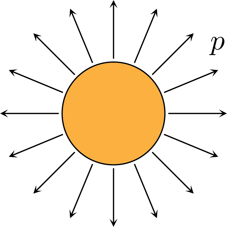
The state of stress which always maintains the same representation with respect to any reference system is the state characterized by principal stresses assuming the same value, that is \(\sigma_1 = \sigma_2 = \sigma_3 = p \text{.}\) In this case, using Eq. (2.4.3), the tensor \(\tens{\sigma} \) takes the following form
Assuming \(p \) positive there is an equal traction in all directions, hence the adjective spherical. On the other hand, if \(p \) is negative, there is a state of compression equal in all directions, just as it happens for a body immersed in a fluid. Hence the adjective hydrostatic.
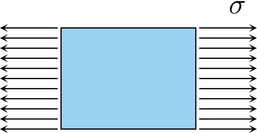
characterized by principal stresses equal to \(\sigma_1 = \sigma \text{,}\)\(\sigma_2 = 0 \text{,}\)\(\sigma_3 = 0 \) and principal directions identified by the axis \(\vec{e}_1 \) and the plane defined by the other two axes of the triad, it is usually labeled, based on the sign of \(\sigma \text{,}\) state of “pure” traction or “pure” compression.
The adjective “pure” must not be misleading as it only applies to the arrangement of principal directions just described. In fact, it is sufficient to assume a different arrangement for the principal directions, for example obtained with a generic rotation around the axis \(\vec{e}_3 \text{,}\) to have
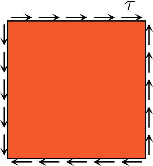
In order to discuss the state of “pure” shear it is necessary to leave the point of view given by the main directions and speak directly of a stress state characterized by the following matrix form
In a such case and always with respect to the given reference triad \(\vec{e}_1\text{,}\)\(\vec{e}_2\text{,}\)\(\vec{e}_3\text{,}\) it is possible to talk of a state of “pure” shear because the only non zero component of the tensor is \(\sigma_{12}=\sigma_{21}=\tau\text{.}\)
The calculation of principal directions and principal stresses would show that we are in a different case from the previous ones. In fact, the calculation of the eigenvalues and eigenvectors can be carried out with the following MATLAB® instructions
Then the principal directions are rotated of \(\pi / 4 \) around the axis \(\vec{e}_3 \) (the normalized eigenvectors are reported even if, in the case of symbolic calculation, MATLAB® does not provide normalized eigenvectors).
as the stress state that occurs when the reference system is obtained by rotating the triad of the main directions of \(\pi/4 \) around the third axis and the principal stresses are defined by