configurations

Section 1.1 configurations

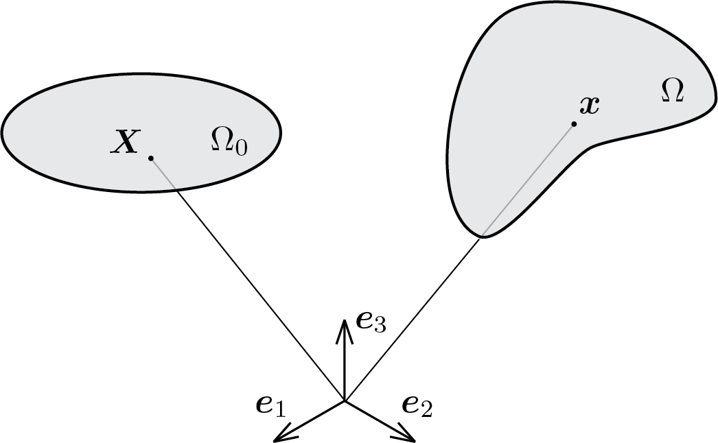
The object of the kinematic analysis is a continuous body which will be named with the symbol \(\body\text{.}\) Each point of the body occupies a position in space which, fixed an orthonormal reference triad \(\vec{e}_a\) (\(a = 1,2,3\)), is identified by a vector. In particular we will talk about two configurations:

the reference configuration \(\body_0\text{,}\) which collects all the positions \(\vec{X}\) occupied by the points of the body before the motion;

🔗
the current configuration \(\body\text{,}\) which collects all the positions \(\vec{x}\) occupied by the points of the body after the motion.

🔗

With respect to the chosen reference base, the positions \(\vec{X}\) and \(\vec{x}\) will be expressed using different types of notation.

\begin{gather*} \left[\begin{array}{c}X_1\\X_2\\X_3\end{array}\right]\,,\quad \left[\begin{array}{c}x_1\\x_2\\x_3\end{array}\right]\\ X_1 \vec{e}_1 + X_2 \vec{e}_2 + X_3 \vec{e}_3\,,\quad x_1 \vec{e}_1 + x_2 \vec{e}_2 + x_3 \vec{e}_3\\ X_a \vec{e}_a\,,\quad x_a \vec{e}_a\,. \end{gather*}

🔗

Below are reported some examples of MATLAB® instructions that can be used to define and manipulate vectors.

🔗

Instructions for creating row vectors.

Listing 1.1.2.

🔗

$ u = [1 2 3]
v = 4:6
w = u + v
x = 0.5
y = 1.0
z = -2.0
k = x*u + y*v + z*w

% how to access to vector's components
u(1)
u(2)
% the same as u(2)
u(1,2)
% access error
u(2,1)

🔗

Instructions for creating column vectors (the format usually adopted to manipulate vectors in Mechanics).

Listing 1.1.3.

🔗

$ u = [1; 2; 3]
v = (linspace(4,6,3))'
w = u + v
x = 0.5
y = 1.0
z = -2.0
k = x*u + y*v + z*w 

% how to access to vector's components
k(1)
k(2)
% the same as k(2)
k(2,1)
% access error
k(1,2)

🔗

Prev Top Next