The solution of the elastic problem under completely generic conditions poses difficulties which are difficult to overcome. Only by making appropriate simplifications, such as for previous examples regarding prismatic solids (simple geometries) and under the action of loads of a precise type, is it possible to obtain an analytical solution of the assigned problem.
The previous considerations and the need to deal with engineering problems concerning solids which, from a geometric point of view, can be modeled through one-dimensional or two-dimensional descriptions, have led to the development of various structural models. These models allow to solve, with an acceptable degree of approximation, various problems that would not be easily tackled using both analytical and numerical tools.
In the following two beam models are presented. They are obtained through a one-dimensional reduction of the solutions found for prismatic solids simply stretched and simply bent, see Table 3.4.6. In particular, we will proceed by showing how it is possible to describe the significant component of the strain, the \(\varepsilon_{33} \text{,}\) referring only to the centerline of the beam, known as beam axis. The component \(\varepsilon_{33} \) is the significant one because it constitutes the only strain component that determines the value of the internal work of the prismatic solid, in fact in the two cases examined we have that
being clear which components we are referring to. So the main purpose is to obtain a description of the internal energy of the one-dimensional model equivalent to the internal energy of the 3D solution taken as a reference.
Furthermore, for the problems examined, the beam axis moves remaining in the plane identified by the axes \(X_3 \) and \(X_2 \) and for this reason the treatment can be carried out in the plane and then we will talk about 2D beam models 1
In the case of the stretched beam the one-dimensional solution should be valid also in a 3D context.
Subsection3.5.2the reference given by the beam axis
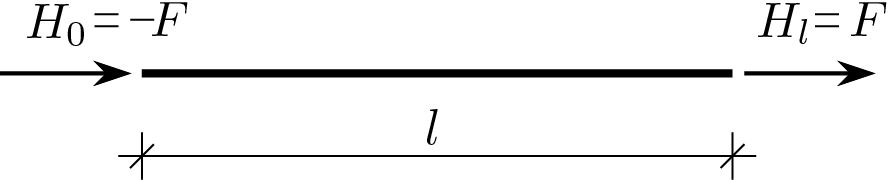
In the case of the prismatic solid that is simply stretched, the beam axis deforms as shown in the Figure, that is, it undergoes a simple elongation or shortening. The figure also highlights the notation that is currently used for this one-dimensional model.
Using the beam axis as a reference, we can calculate the strain component \(\varepsilon_{33} \text{,}\) here simply referred to as \(\varepsilon \text{,}\) simply deriving the displacement variable along the axis
\begin{equation}
L_i = \int_{l} N \varepsilon \,dx\,.\tag{3.5.3}
\end{equation}
The introduced quantity
\begin{equation}
N =\int_{A} \sigma \, dS\,,\tag{3.5.4}
\end{equation}
is the static entity that in the one-dimensional reduction performs the internal work on strain. \(N\) is called axial force and is measured as a force, \(\left[\text{F}\right]\text{.}\)
Relationship that highlights how the proportionality coefficient that defines the link between \(N \) and \(\varepsilon \) is given by the product between the Young’s modulus of the material and the cross-section area of the beam.
Up to this point the one-dimensional reduction has remained strictly adherent to the 3D solution from which we started. If we continue on the same false line also for external loads you will get the following situation
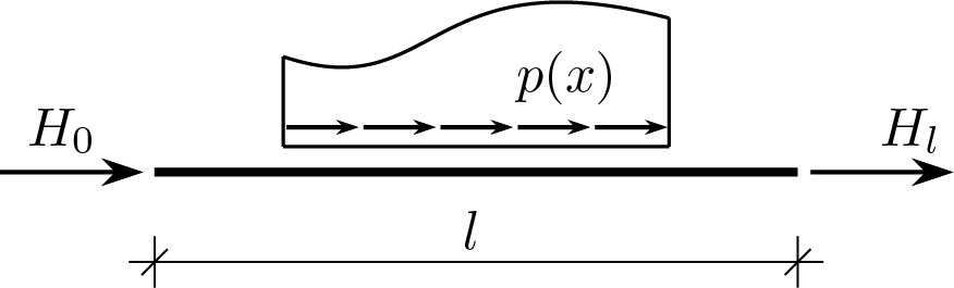
With the definition of the external loads admissible for the beam model, the choice is made instead of extending the use of the model also to cases that in general are not included in the solution of the simply stretched prismatic solid. In particular, as the following Figure shows,
we introduce the load per unit of length \(\func{p}{x} \text{,}\) a generic function dependent on the abscissa \(x \text{,}\) and the concetrated end forces, however expected, are generally different. The external work therefore assumes the following expression
Furthermore, unlike the reference 3D solution, the choice of the admissible loads determines for \(\func{u}{x} \) a pattern which is no longer limited to linear variability alone. The normal stress and axial strain, constant in the reference solution, also become generic functions of the type \(\func{N}{x} \) and \(\func{\varepsilon}{x}\text{.}\)
Subsection3.5.6virtual work principle and equilibrium equations
At this point the definition of the model is practically complete. Only the definition of equilibrium equations, which can be obtained through the virtual work principle, is missing. The principle can be formulated as follows
The relationship just written, where we have neglected to make explicit the dependencies on the variable \(x \text{,}\) can be manipulated by carrying out the following steps
As regards the boundary conditions, it is worth to be noted that on each end it is possible to assign either a static condition or a kinematic condition.
Equilibrium equation can be manipulated in order to obtain an expression in which the displacement \(\func{u}{x} \) appears as unknown. In particular by carrying out the following steps
\begin{align*}
\frac{dN}{d x} + p \amp= 0\\
\frac{d}{d x}\left(EA\,\varepsilon\right) + p \amp= 0\\
\frac{d}{d x}\left(EA\,\frac{du}{dx}\right) + p \amp= 0
\end{align*}
the following result is obtained
\begin{equation}
EA\,\frac{d^2u}{dx^2} + p = 0\,.\tag{3.5.21}
\end{equation}