The elastic modeling of uniaxial states, i.e. states of tension and deformation in which only one stress component and the associated strain component are present, can be carried out through a direct application of Hooke’s law.
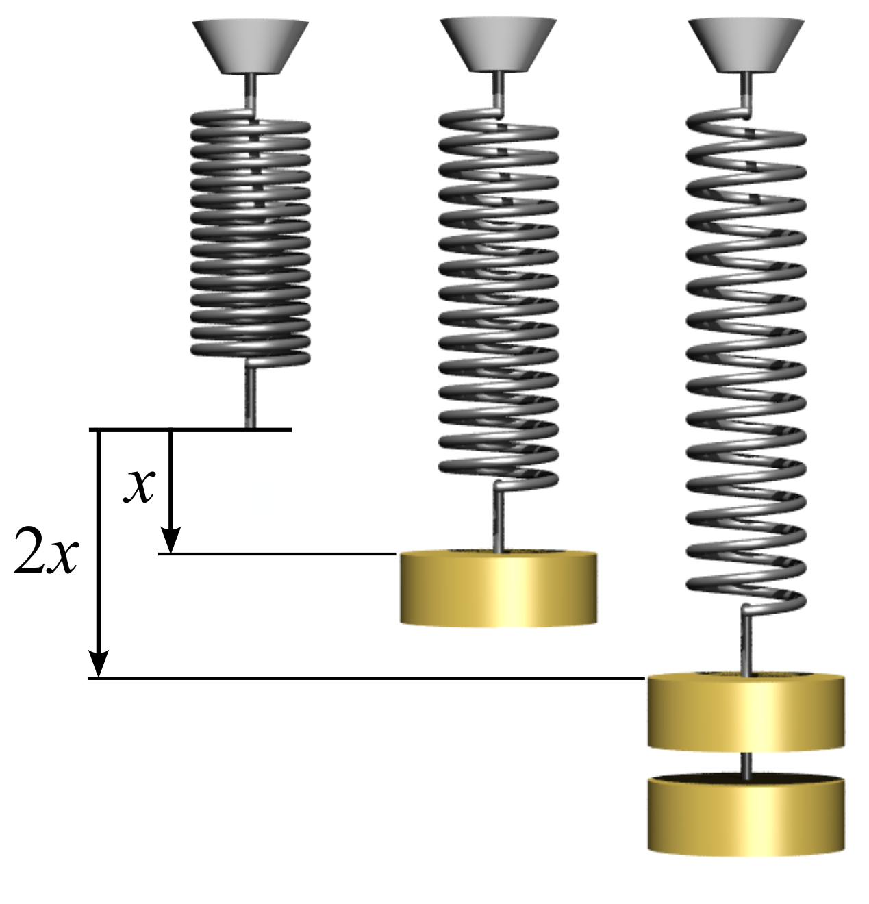
Hooke’s law is a law of physics which states that the force \(F \) needed to extend or compress a spring by an amount \(x \) scales linearly with respect to that amount, i.e.
\begin{equation}
F = k\,x\,.\tag{3.2.1}
\end{equation}
\(k\;\left[\frac{\text{N}}{\text{m}}\right]\) is known as stiffness and is a parameter, characteristic of the spring, constant and positive, \(x\;\left[\text{m}\right]\) is the elongation that the spring undergoes (in the case of a negative \(x\) the spring undergoes a shortening).
The law is named after the 17th century British physicist Robert Hooke who first made the law public in 1676 as a Latin anagram. Subsequently, in 1678, he published the solution of his anagram as: ut tensio, sic vis (the extension is proportional to the force).
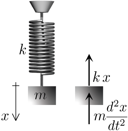
In order to highlight also the concept of elastic energy stored by the spring due to the effect of elongation \(x \text{,}\) consider the following mechanical scheme where all the forces acting have been highlighted (for simplicity let’s suppose to carry out the experiment in the absence of gravity 1
In fact if we also took gravity into account the nature of the resulting equation would not change.
and dissipative forces) on a body of mass \(m \) and constrained by a stiffness spring \(k \text{.}\)
Due to the displacement \(x \) measured from the equilibrium position, the body is subject to the inertia force \(m \, \frac {d^2 x} {dt^2} \) and the elastic force \(k \, x \) directed as shown in the figure. For the balance of the system we have
The differential equation obtained characterizes a system which, in mechanics, is called simple harmonic oscillator. The solution of the differential equation is described by the function
where \(\func{x}{0}\) and \(\func{\frac{dx}{dt}}{0}\) represent the initial positon and velocity. \(\omega \) is called pulsation and is measured in \(\left[\frac{\text{rad}}{\text{s}}\right]\text{.}\)
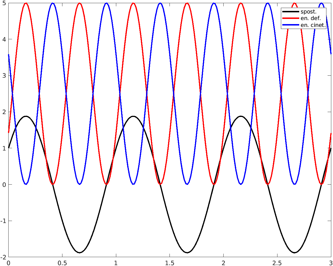
By way of example, the MATLAB® instructions that can be used for plotting the function on the basis of the following data are reported: \(\omega = 2\pi\;\left[\frac{\text{rad}}{\text{s}}\right]\text{,}\)\(m=10\;\left[\text{kg}\right]\text{,}\)\(\func{x}{0}= 1 \; \left[\text{m}\right]\) and \(\func{\frac{dx}{dt}}{0}= 10 \; \left[\frac{\text{m}}{\text{s}}\right]\text{.}\)Listing3.2.4.
and it shows, in graphic form, the continuous transformation of the elastic energy of the spring into kinetic energy of the body and vice versa. The elastic energy (red color) oscillates between zero and the maximum value that occurs when the absolute value of the displacement (black color) is maximum, at the same time the velocity is zero. On the contrary, the kinetic energy (blue color) is maximum when the absolute value of the velocity is maximum, when at the same instant the displacement is zero.
To conclude, it is observed that the elastic energy acts as a potential for the elastic force of the spring as the latter can be obtained by deriving the energy, i.e.
\begin{equation*}
F = \frac{d}{dx}\left( \frac{1}{2}k\,x^2 \right) = k\, x\,.
\end{equation*}
Subsection3.2.1uniaxial tensile or compressive test
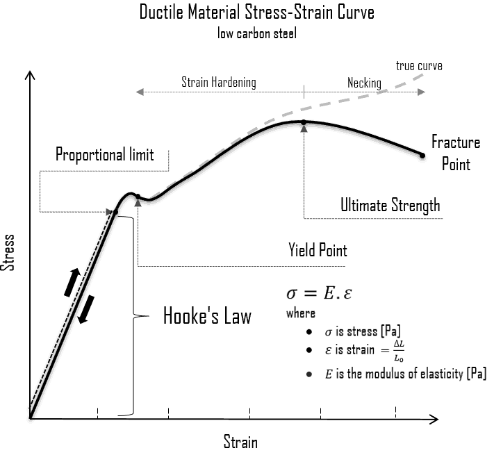
The following figure illustrates the result of an uniaxial load test performed on a steel bar. The result of the test is the curve shown in the figure, a curve that represents the mechanical response, that is, the value of the stress in the material, as the applied deformation increases. It is evident how the response of the material is articulated and variable and how it is not trivial to identify a mathematical / numerical model capable of reproducing the result produced by the load test, a result that can be schematically summarized as follows (for steel, and in general for metallic materials, what is shown in the figure is generally assumed to be valid both under traction and compression).
There is a limit to the linear phase (Proportional limit) beyond which the response tends to remain constant by staying in the phase called yielding (Yield Point).
The focus of this chapter is however only the first phase of the response of the material, a phase that is not only linear but also elastic in the sense that Hooke’s law is applicable and therefore among the only components of tension and deformation, \(\sigma \) and \(\varepsilon \text{,}\) present in an uniaxial condition, it is legitimate to assume that the following proportional relationship exists
The symbol \(E \) is used to denote the Young’s modulus which is a specific characteristic of the material and is measurable with a load test of the type described above (trivially \(E \) is given by the slope that the response curve assumes in the elastic phase). Recalling that the deformation is dimensionless the unit of measurement used for \(E \) is identical to that used for the stress \(\ sigma \text{.}\) Some examples of units of measurement used are the following
What has been observed for the uniaxial tensile test also occurs in the uniaxial tests which involve tangential components of stress and strain. Again there is a first part of the response that can be described trough Hooke’s law. However, the proportionality coefficient changes. In particular, the relationship between the tangential stress component \(\tau \) and the shear deformation component \(\gamma \) (see (1.9.10)) can be formulated as follows