generalized section forces calculation and diagrams

Section 5.9 generalized section forces calculation and diagrams

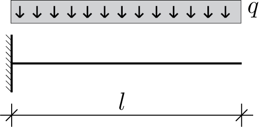
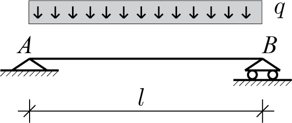
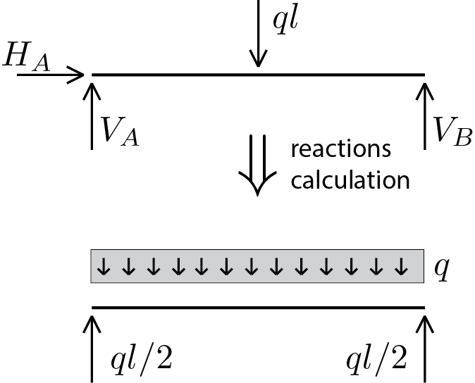
The static analysis presented in the previous sections allows to evaluate the constraint reactions for an isostatic system. Starting from this information and using general integrals (5.8.13), (5.8.14) and (5.8.15) it is possible to proceed with the calculation of the generalized section forces for beams subjected to generic forces / torques and at most constant distributed loads (for generic distributed loads it is necessary to use the (5.8.10), (5.8.11) and (5.8.12)).

🔗

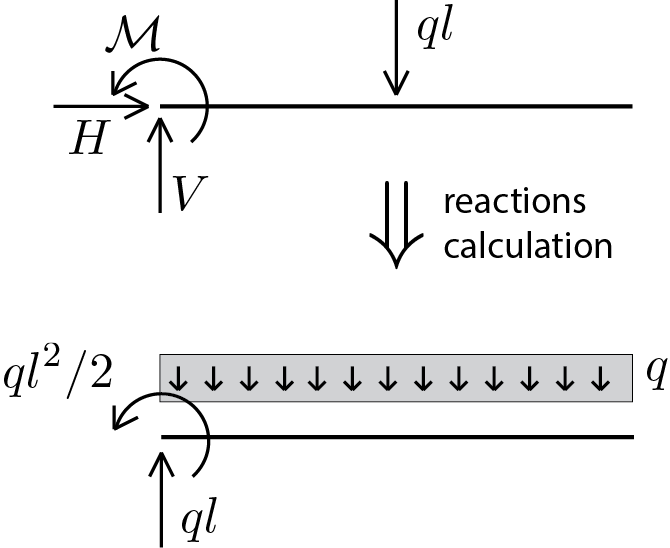
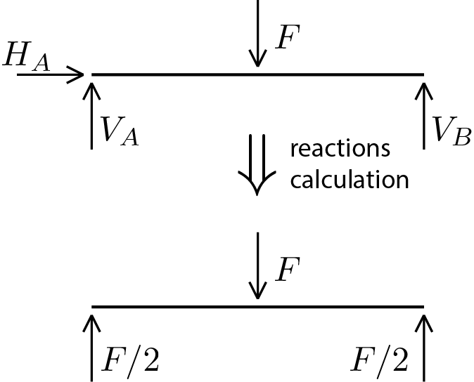
The calculation procedure will be illustrated by discussing some examples and using MATLAB® to carry out the required calculations and display the results. Given the simplicity of the schemes considered, the explicit calculation of the constraint reactions is omitted.

🔗

Subsection 5.9.1

Consider the following free body diagram whose satisfaction of the equilibrium conditions is easy to be checked.

🔗

It is evident from the diagram that the values assumed by the section forces for \(x = 0 \) are

\begin{equation*} N(0) = F\,,\quad T(0) = F\,,\quad M(0) = -F l\,. \end{equation*}

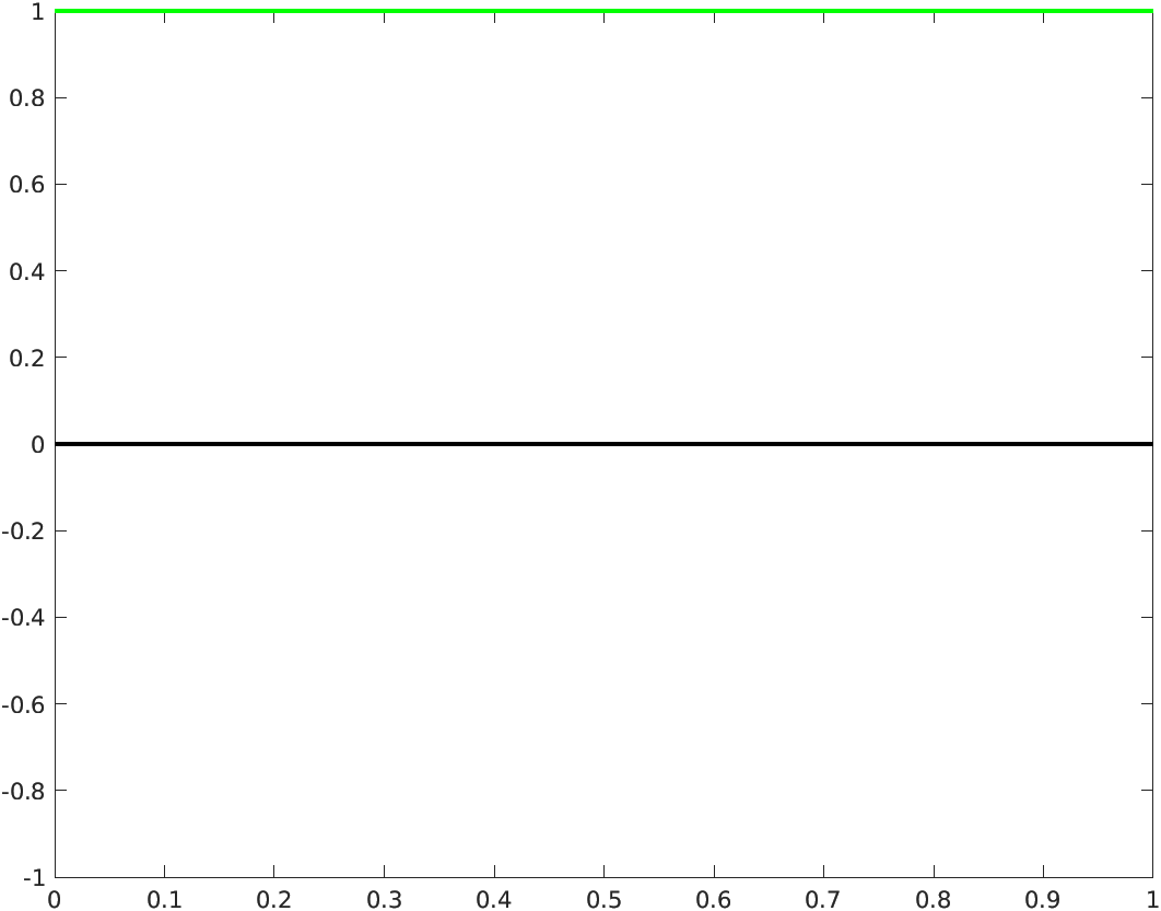
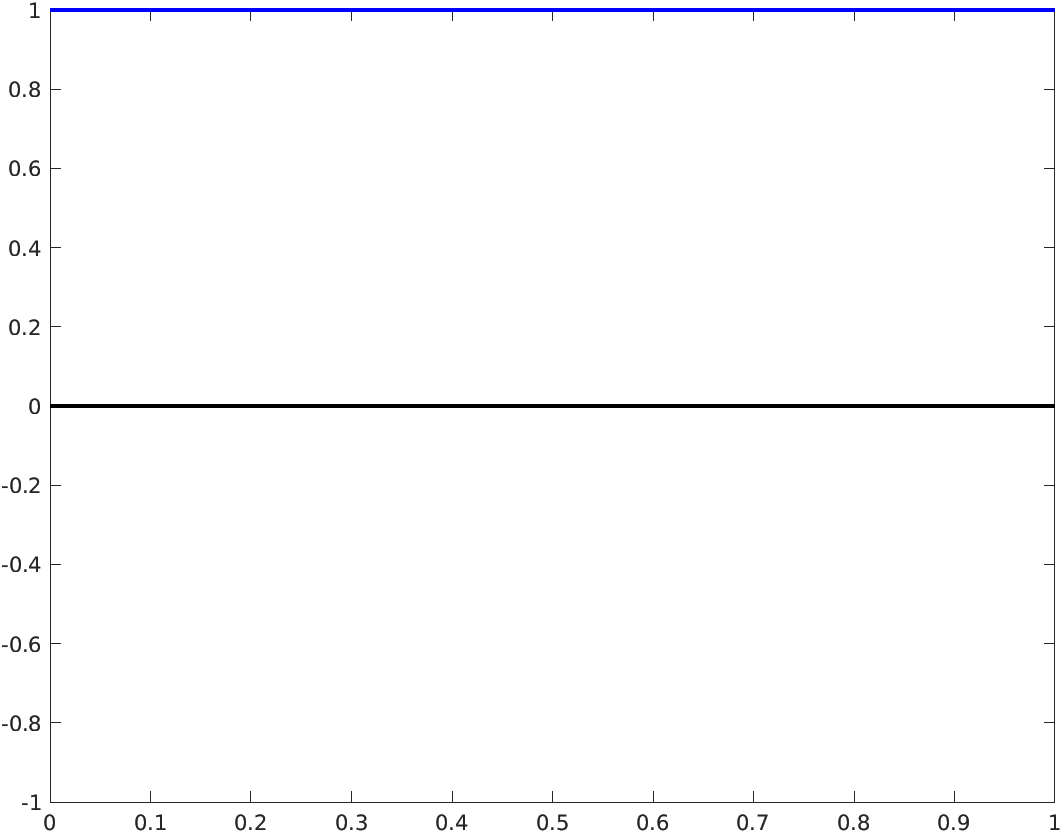
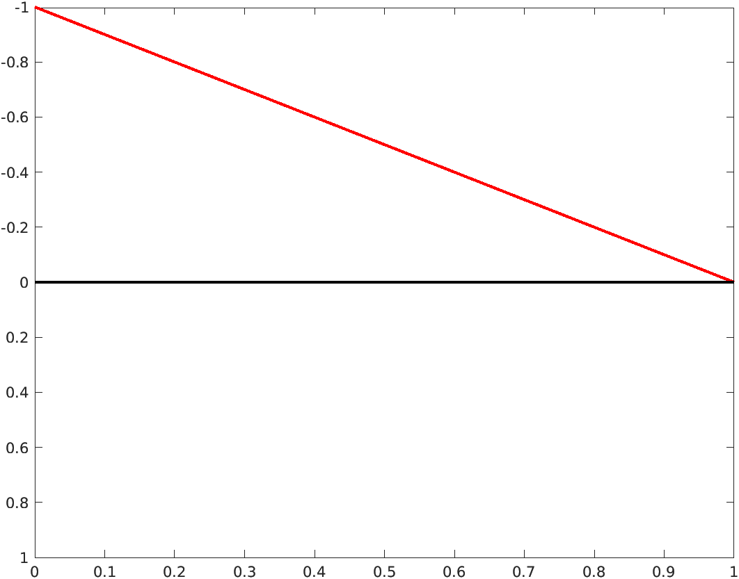
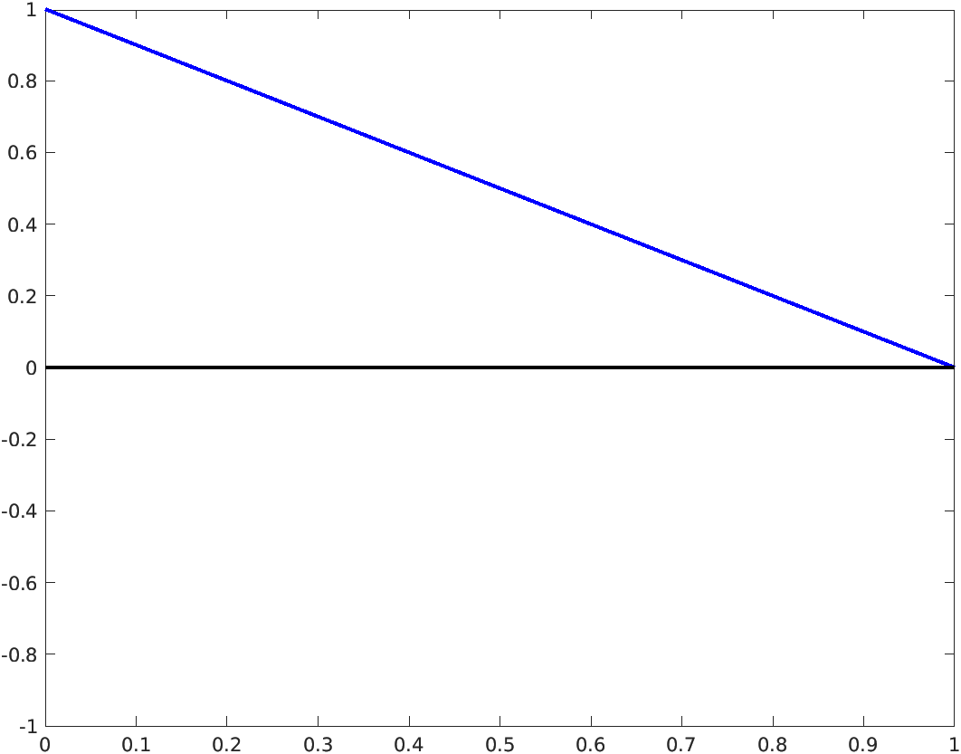
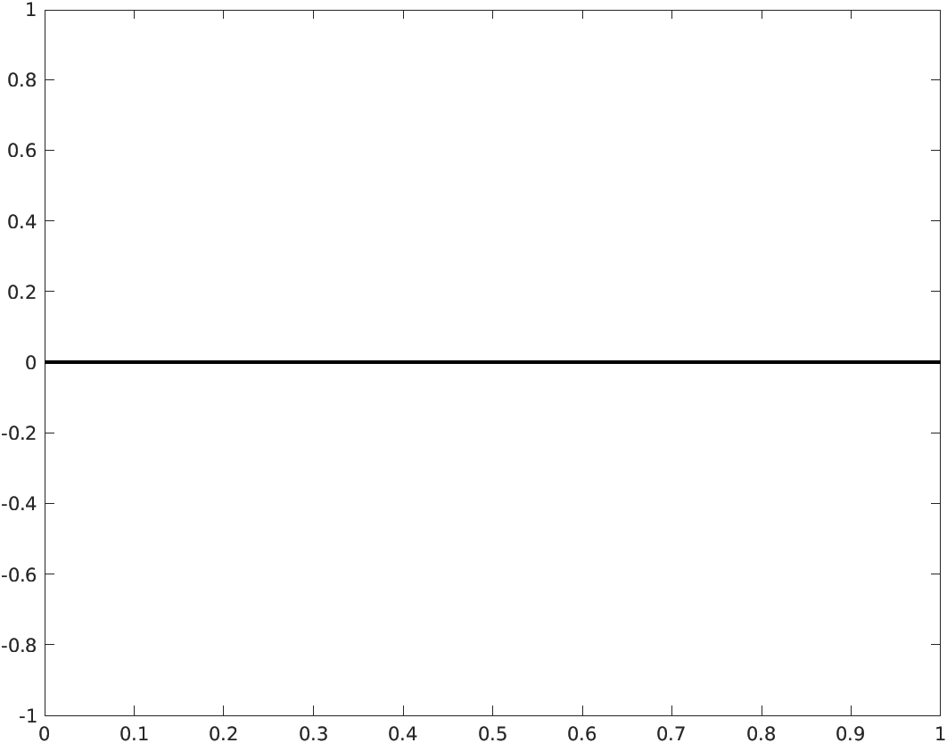
Using the general integrals, we obtain the following expressions of the generalized section forces as a function of the abscissa \(x \) placed along the axis of the beam

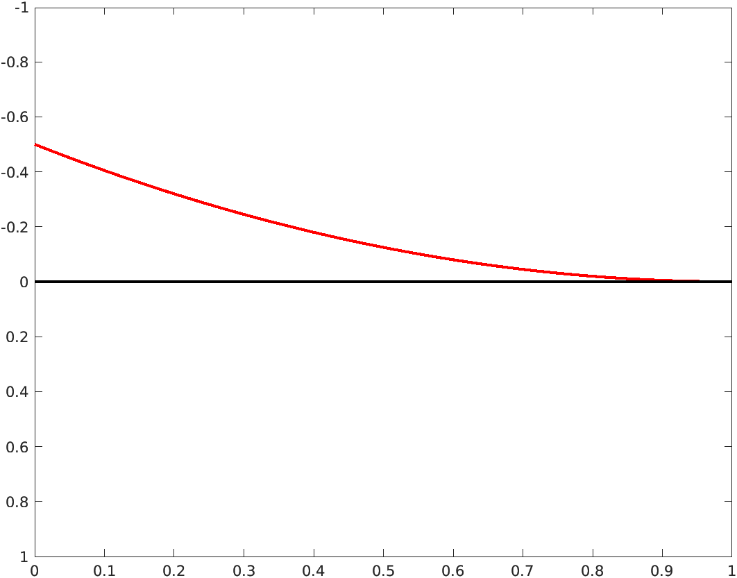
\begin{equation*} N(x) = F\,,\quad T(x) = F\,,\quad M(x) = -F l + F\,x\,. \end{equation*}

🔗

The latter results can be plotted using the following MATLAB® instructions.

Listing 5.9.2.

🔗

$ % axial force diagram
syms N(x, F);
N(x,F) = F;

np = 100;
Xv = 0:1/np:1;
Nv = N(Xv, 1);
Beam = zeros(1, np+1);

plot(Xv,Nv,'g',Xv,Beam,'k','LineWidth',2)
set(gca, 'Ylim', [-1 1])


% shear force diagram
syms T(x,F);
T(x,F) = F;

np = 100;
Xv = 0:1/np:1;
Tv = T(Xv, 1);
Beam = zeros(1, np+1);

plot(Xv,Tv,'b',Xv,Beam,'k','LineWidth',2)
set(gca, 'Ylim', [-1 1])


% bending moment diagram
syms M(x,F,l);
M(x,F,l) = -F*l + F*x;

np = 100;
Xv = 0:1/np:1;
Mv = M(Xv, 1, 1);
Beam = zeros(1, np+1);

plot(Xv,Mv,'r',Xv,Beam,'k','LineWidth',2)
set(gca, 'Ylim', [-1 1])
set(gca, 'YDir','reverse')

🔗

In this way we obtain the following diagrams for axial force (green), shear force (blue) and bending moment (red).

🔗

Note how the representation of the bending moment is carried out by changing the direction of the vertical axis of the diagram. This choice is used in professional practice to "visualize" which of the two edges of the beam, lower or upper, is under tensile condition.

🔗

Subsection 5.9.2

Let us consider the following scheme regarding a cantilever beam subjected to a constant distributed load.

🔗

The free body diagram and the related computation of the constraint reactions provide the following result.

🔗

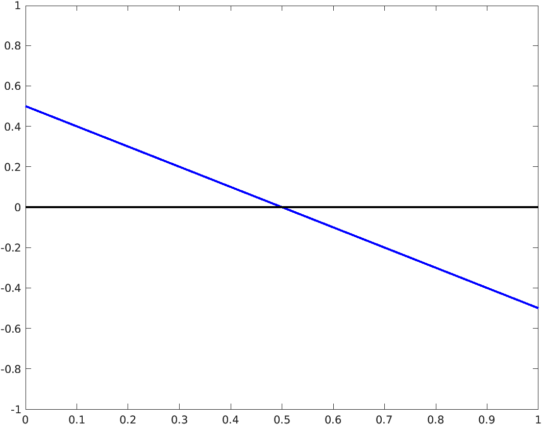
Information that can be used in writing general integrals (5.8.13), (5.8.14), (5.8.15), and obtain the following expression of the generalized section forces along the beam axis .

\begin{equation*} N(x) = 0\,,\quad T(x) = -q\,x + ql \,,\quad M(x) = -ql^2/2 + ql\,x - q\,x^2/2 \,. \end{equation*}

🔗

The latter results can be plotted using the following MATLAB® instructions.

Listing 5.9.5.

🔗

$ % axial force diagram
syms N(x);
N(x) = 0;

np = 100;
Xv = 0:1/np:1;
Nv = N(Xv);
Beam = zeros(1, np+1);

plot(Xv,Nv,'g',Xv,Beam,'k','LineWidth',2)
set(gca, 'Ylim', [-1 1])


% shear force diagram
syms T(x,q,l);
T(x,q,l) = -q*x+q*l;

np = 100;
Xv = 0:1/np:1;
Tv = T(Xv, 1, 1);
Beam = zeros(1, np+1);

plot(Xv,Tv,'b',Xv,Beam,'k','LineWidth',2)
set(gca, 'Ylim', [-1 1])


% bending moment diagram
syms M(x,q,l);
M(x,q,l) = -q*l^2/2 + q*l*x - q*l*x^2/2;

np = 100;
Xv = 0:1/np:1;
Mv = M(Xv, 1, 1);
Beam = zeros(1, np+1);

plot(Xv,Mv,'r',Xv,Beam,'k','LineWidth',2)
set(gca, 'Ylim', [-1 1])
set(gca, 'YDir','reverse')

🔗

Subsection 5.9.3

Let us consider a supported beam subjected to a distributed load.

🔗

Constraint reactions are calculated through the free body diagram as follows.

🔗

The obtained solution allows the writing of the following conditions regarding to the end \(A \) of the beam

\begin{equation*} N(0) = 0\,,\quad T(0) = ql/2\,,\quad M(0) = 0\,, \end{equation*}

from which it is easy to obtain the expression of generalized section forces along the beam:

\begin{equation*} N(x) = 0\,,\quad T(x) = -q\,x + ql/2 \,,\quad M(x) = ql/2\,x - q\,x^2/2 \,. \end{equation*}

🔗

It is now possible to plot the diagrams of obtained generalized section forces.

Listing 5.9.8.

🔗

$ % axial force diagram
syms N(x);
N(x) = 0;

np = 100;
Xv = 0:1/np:1;
Nv = N(Xv);
Beam = zeros(1, np+1);

plot(Xv,Nv,'g',Xv,Beam,'k','LineWidth',2)
set(gca, 'Ylim', [-1 1])


% shear force diagram
syms T(x,q,l);
T(x,q,l) = -q*x+q*l/2;

np = 100;
Xv = 0:1/np:1;
Tv = T(Xv, 1, 1);
Beam = zeros(1, np+1);

plot(Xv,Tv,'b',Xv,Beam,'k','LineWidth',2)
set(gca, 'Ylim', [-1 1])


% bending moment diagram
syms M(x,q,l);
M(x,q,l) = q*l/2*x - q*l*x^2/2;

np = 100;
Xv = 0:1/np:1;
Mv = M(Xv, 1, 1);
Beam = zeros(1, np+1);

plot(Xv,Mv,'r',Xv,Beam,'k','LineWidth',2)
set(gca, 'Ylim', [-1 1])
set(gca, 'YDir','reverse')

🔗

Subsection 5.9.4

Let us consider a supported beam subjected to a concentrated force in the middle point.

🔗

The evaluation of the constraint reactions furnishes the following result.

🔗

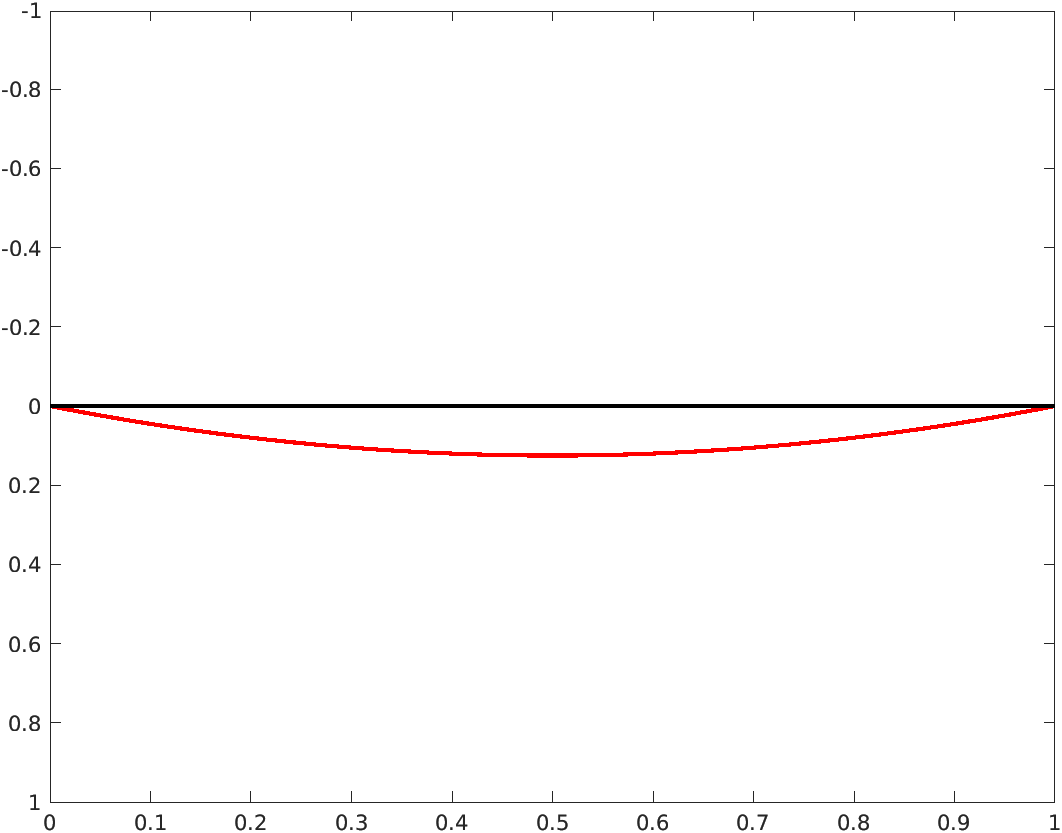
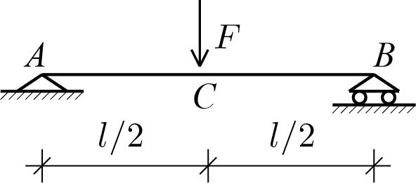
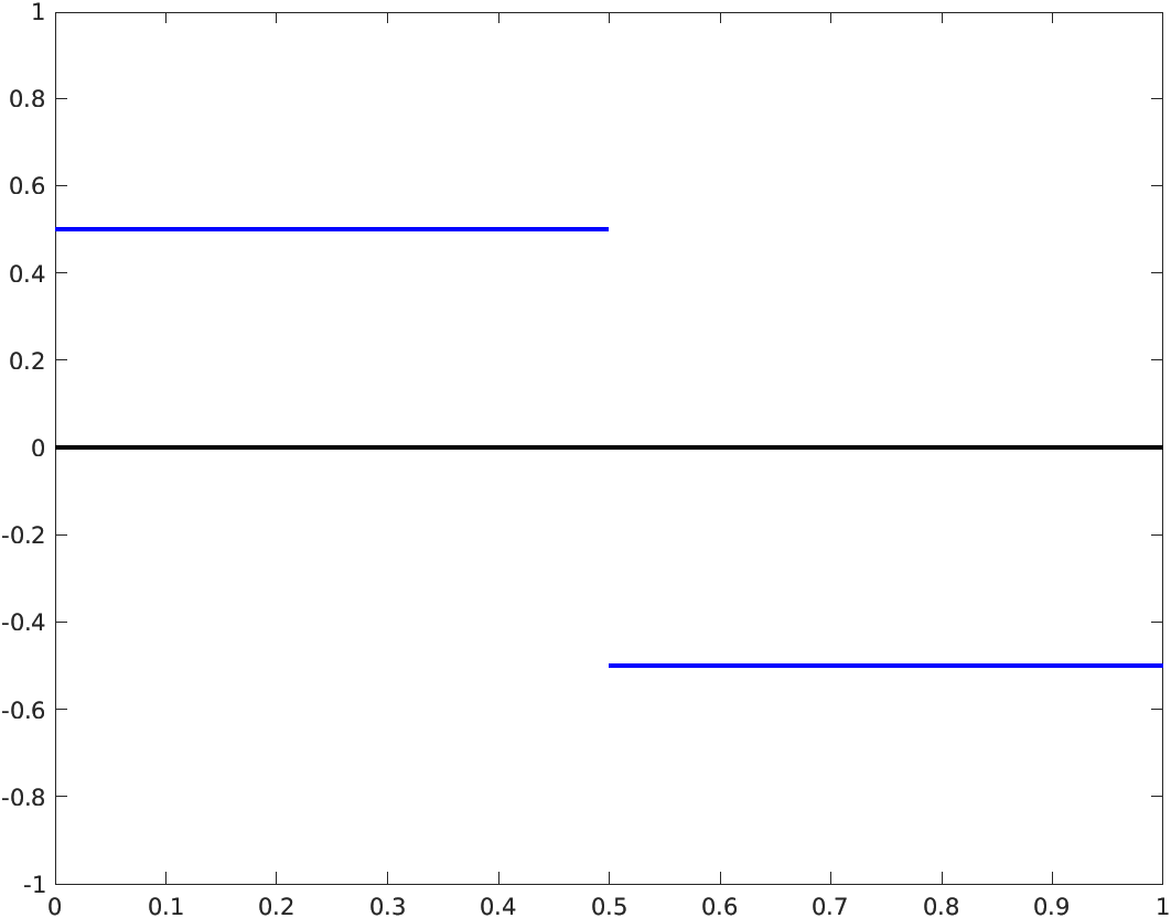
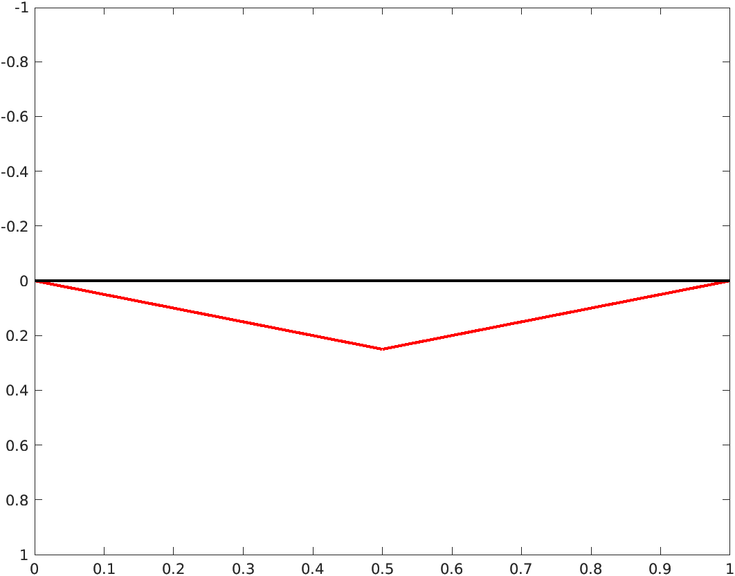
Compared to the previous cases, the current case is different because the force concentrated in the middle determines a discontinuity of the shear \(T (x) \) and therefore, being \(dM / dx = T \text{,}\) also a discontinuity of the derivative of the bending moment. Therefore the general integrals (5.8.13), (5.8.14) and (5.8.15) are not directly applicable to whole beam \(AB \) but they must be applied separately to the \(AC \) and \(CB \) beam portions. In this way, two descriptions of \(T (x) \) and \(M (x) \) are obtained, one description valid for the \(AC \) portion and the other one valid for the \(CB \) portion.

\(AC\) portion, \(0 \leq x \leq l/2\text{:}\)
\begin{align*} N_{AC}(0) &= 0\,,\\ T_{AC}(0) &= F/2\,,\\ M_{AC}(0) &= 0\,. \end{align*}
which give
\begin{align*} N_{AC}(x) &= 0\,,\\ T_{AC}(x) &= F/2\,,\\ M_{AC}(x) &= F/2\,x\,. \end{align*}

🔗
\(CB\) portion, \(0 \leq x \leq l/2\text{:}\)
\begin{align*} N_{CB}(0) &= 0\,,\\ T_{CB}(0) &= T_{AC}(l/2) - F=F/2-F=-F/2\,,\\ M_{CB}(0) &= M_{AC}(l/2) = Fl/4\,. \end{align*}
which give
\begin{align*} N_{CB}(x) &= 0\,,\\ T_{CB}(x) &= -F/2\,,\\ M_{CB}(x) &= -F/2\,x + Fl/4\,. \end{align*}

🔗

🔗

Listing 5.9.11.

🔗

$ % shear force diagram
syms T_ac(x,F) T_cb(x,F);
T_ac(x,F) = F/2;
T_cb(x,F) = -F/2;

np = 50;
Xv = 0:0.5/np:0.5;
Tv_ac = T_ac(Xv, 1);
Tv_cb = T_cb(Xv, 1);

Xv_ac = Xv;
Xv_cb = 0.5:0.5/np:1;
Beam = zeros(1, np+1);

plot(Xv_ac,Tv_ac,'b', Xv_ac,Beam,'k', ...
Xv_cb,Tv_cb,'b', Xv_cb,Beam,'k', 'LineWidth',2)
set(gca, 'Ylim', [-1 1])


% bending moment diagram
syms M_ac(x,F) M_cb(x,F,l);
M_ac(x,F) = F/2*x;
M_cb(x,F,l) = -F/2*x+F*l/4;

np = 50;
Xv = 0:0.5/np:0.5;
Mv_ac = M_ac(Xv, 1);
Mv_cb = M_cb(Xv, 1, 1);

Xv_ac = Xv;
Xv_cb = 0.5:0.5/np:1;
Beam = zeros(1, np+1);

plot(Xv_ac,Mv_ac,'r', Xv_ac,Beam,'k', ...
Xv_cb,Mv_cb,'r', Xv_cb,Beam,'k', 'LineWidth',2)
set(gca, 'Ylim', [-1 1])
set(gca, 'YDir','reverse')

🔗

Prev Top Next