
Section 3.8 applications of the bent beam model

Subsection 3.8.1 cantilever beam subjected to a shear force at the free end

Figure 3.8.1.

Applying the equilibrium equation (3.6.34) to the above scheme provides

\begin{equation*} EJ\,\frac{d^4w}{dx^4} = 0\,. \end{equation*}

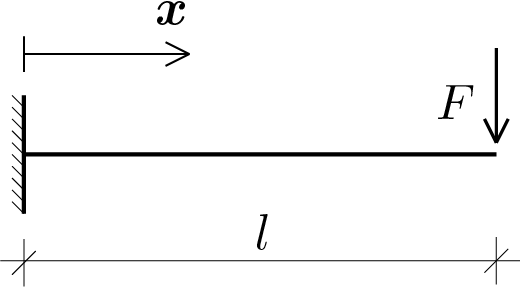
A fourth order differential equation to be solved with respect to boundary conditions which, for the present case, are kinematic conditions at the end \(x=0\) and static conditions at the end \(x=l\) 1 :

\begin{align*} \amp \func{w}{0} = 0\,,\\ \amp \func{\frac{dw}{dx}}{0} = 0\,,\\ \amp \func{\frac{d M}{dx}}{l} = \frac{d}{dx}\left(-EJ\,\func{\frac{d^2w}{dx^2}}{l}\right) = -EJ\,\func{\frac{d^3w}{dx^3}}{l} = F\,,\\ \amp \func{M}{l} = -EJ\,\func{\frac{d^2w}{dx^2}}{l} = 0\,. \end{align*}
In general at one end the conditions can be also mixed, kinematic and static.

The following MATLAB® instructions allow the calculation of the solution \(\func{w}{x} \) and its bending moment \(\func{M}{x}\text{.}\)

syms w(x) EJ F l;
ode = EJ*diff(w,x,4) == 0;
D1w = diff(w,x,1);
D2w = diff(w,x,2);
D3w = diff(w,x,3);
cond1 = w(0) == 0;
cond2 = D1w(0) == 0;
cond3 = -EJ*D3w(l) == F;
cond4 = -EJ*D2w(l) == 0;
conds = [cond1 cond2 cond3 cond4];
sol = dsolve(ode,conds)
M = -EJ*diff(sol,x,2)
Listing 3.8.2.

the deformed configuration of the beam axis can be plotted by using the following MATLAB® instructions.

syms w(x);
EJ = 1;
F = 1;
l = 1;
w(x)=F/6/EJ*(-x^3+3*l*x^2);

np = 100;
Xv = 0:1/np:1;
wv = w(Xv);
Beam = zeros(1, np+1);
plot(Xv,wv,'r',Xv,Beam,'k','LineWidth',2)
set(gca, 'YDir','reverse')
Listing 3.8.3.

The expected cubic pattern is therefore obtained for the displacement

\begin{equation*} \func{w}{x} = \frac{F}{6\,EJ}\left(-x^3+3l\,x^2\right)\,, \end{equation*}

and for the bending moment there is instead the following linear solution

\begin{equation*} \func{M}{x} = F\left(x-l\right)\,. \end{equation*}

Subsection 3.8.2 cantilever beam subjected to a constant distributed load

Figure 3.8.4.

In the present case differential equation (3.6.34) gives

\begin{equation*} -EJ\,\frac{d^4w}{dx^4} + q = 0\,, \end{equation*}

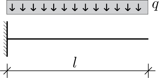
where the applied transversal distributed load is constant. Also in this case the boundary conditions are kinematic conditions at \(x=0\) and static conditions at \(x=l\text{:}\)

\begin{align*} \amp \func{w}{0} = 0\,,\\ \amp \func{\frac{dw}{dx}}{0} = 0\,,\\ \amp \func{\frac{d M}{dx}}{l} = \frac{d}{dx}\left(-EJ\,\func{\frac{d^2w}{dx^2}}{l}\right) = -EJ\,\func{\frac{d^3w}{dx^3}}{l} = 0\,,\\ \amp \func{M}{l} = -EJ\,\func{\frac{d^2w}{dx^2}}{l} = 0\,. \end{align*}

The above equations, equilibrium and related boundary conditions, can be formulated in MATLAB® as follows, allowing the calculation of the solution \(\func{w}{x} \) and of the relative bending moment \(\func{M}{x}\text{.}\) Instructions for plotting the two functions are also provided. funzioni.

syms w(x) EJ q l;
ode = -EJ*diff(w,x,4) + q == 0;
D1w = diff(w,x,1);
D2w = diff(w,x,2);
D3w = diff(w,x,3);
cond1 = w(0) == 0;
cond2 = D1w(0) == 0;
cond3 = -EJ*D3w(l) == 0;
cond4 = -EJ*D2w(l) == 0;
conds = [cond1 cond2 cond3 cond4];
sol(x,EJ,q,l) = dsolve(ode,conds)
M(x,EJ,q,l) = -EJ*diff(sol,x,2)

np = 100;
Xv = 0:1/np:1;
wv = sol(Xv,1,1,1);
Beam = zeros(1, np+1);
plot(Xv,wv,'r',Xv,Beam,'k','LineWidth',2)
set(gca, 'YDir','reverse')

Mv = M(Xv,1,1,1);
plot(Xv,Mv,'b',Xv,Beam,'k','LineWidth',2)
set(gca, 'YDir','reverse')
Listing 3.8.5.

Subsection 3.8.3 supported beam subjected to a constant distributed load

Figure 3.8.6.

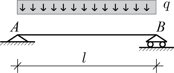
The solution to the problem is obtained on the basis of the same equilibrium equation used in the previous example. It is only necessary to modify the boundary conditions which, for the supported beam, become

\begin{align*} \amp \func{w}{0} = 0\,,\\ \amp \func{M}{0} = -EJ\,\func{\frac{d^2w}{dx^2}}{0} = 0\,.\\ \amp \func{w}{l} = 0\,,\\ \amp \func{M}{l} = -EJ\,\func{\frac{d^2w}{dx^2}}{l} = 0\,, \end{align*}

where static and kinematic conditions are mixed at each beam end.

Similarly, the MATLAB® instructions for calculating the solution change only in the part concerning boundary conditions.

syms w(x) EJ q l;
ode = -EJ*diff(w,x,4) + q == 0;
D1w = diff(w,x,1);
D2w = diff(w,x,2);
D3w = diff(w,x,3);
cond1 = w(0) == 0;
cond2 = -EJ*D2w(0) == 0;
cond3 = w(l) == 0;
cond4 = -EJ*D2w(l) == 0;
conds = [cond1 cond2 cond3 cond4];
sol(x,EJ,q,l) = dsolve(ode,conds)
M(x,EJ,q,l) = -EJ*diff(sol,x,2)

np = 100;
Xv = 0:1/np:1;
wv = sol(Xv,1,1,1);
Beam = zeros(1, np+1);
plot(Xv,wv,'r',Xv,Beam,'k','LineWidth',2)
set(gca, 'YDir','reverse')

Mv = M(Xv,1,1,1);
plot(Xv,Mv,'b',Xv,Beam,'k','LineWidth',2)
set(gca, 'YDir','reverse')
Listing 3.8.7.