
Section 1.6 polar decomposition

The possibility that a given linear transformation may be the result of the composition of several linear transformations and the physical consideration that the motion of a body is made up of elementary transformations such as rotation and pure deformation, lead to the following fundamental result.

polar decomposition theorem.

Given the deformation gradient \(\func{\tens{F}}{\vec{X}}\text{,}\) there is a single polar decomposition at each point defined as follows

\begin{equation} \tens{F} = \tens{R}\tens{U} = \tens{V}\tens{R}.\label{polar_dec_eq}\tag{1.6.1} \end{equation}

\(\tens{R}\) is the rotation tensor, then an orthogonal proper tensor, which satisfies the relationship

\begin{equation} \transp{\tens{R}}\tens{R} = \tens{I}\,.\tag{1.6.2} \end{equation}

\(\tens{U}\) and \(\tens{V}\) are the right stretch tensor and the left stretch tensor, rispectively. These tensors are unique, positive definite and symmetric. Positive definiteness imposes that for any vector \(\vec{v} \neq \vec0\) the satisfaction of the following property

\begin{equation} \vec{v} \cdot \left(\tens{U} \vec{v} \right) > 0 \,,\qquad \vec{v} \cdot \left(\tens{V} \vec{v} \right) > 0\,,\tag{1.6.3} \end{equation}

while symmetry implies

\begin{equation} \tens{U} = \transp{\tens{U}}\,,\qquad \tens{V} = \transp{\tens{V}}\,.\tag{1.6.4} \end{equation}
Remark 1.6.1.

The application of the right polar decomposition to (1.3.9) furnishes

\begin{equation} d\vec{x} = \tens{F}\, d\vec{X} = \tens{R}\, \left(\tens{U}\, d\vec{X}\right) \,,\tag{1.6.5} \end{equation}

which shows how the vector \(d\vec{X}\) is first stretched and after rotated. By applying the left polar decomposition it is obtained

\begin{equation} d\vec{x} = \tens{F}\, d\vec{X} = \tens{V}\, \left(\tens{R}\, d\vec{X}\right) \,,\tag{1.6.6} \end{equation}

to be interpreted as a deformation sequence of \(d\vec{X}\) followed by a rotation. What has been said is illustrated by the following figure.

Figure 1.6.2.
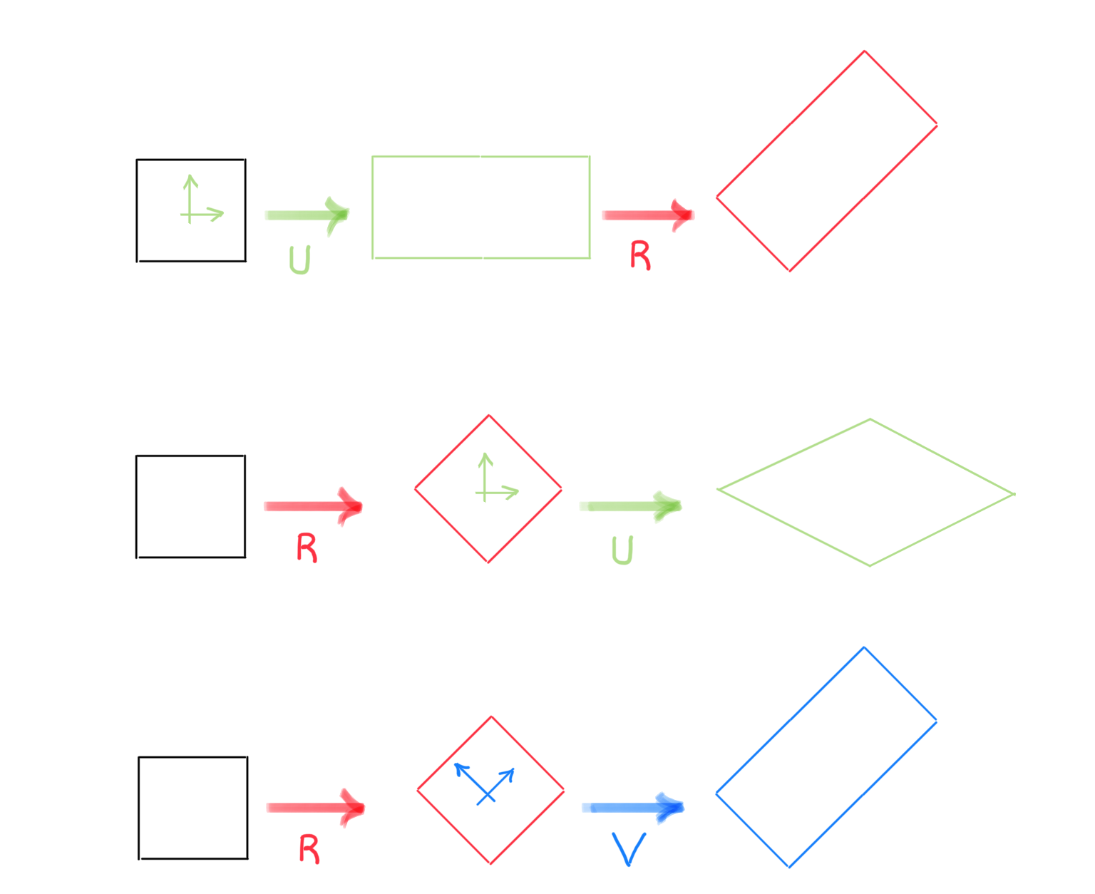
In particular, we illustrate the case in which the right stretch tensor, \(\tens{U} \text{,}\) produces only an elongation in the horizontal direction and, subsequently, the tensor \(\tens{R} \) produces a rotation of 45 \(^o\text{.}\) It is evident that if the rotation is applied first, second and third transformation sequence in the figure, the stretch tensor cannot be the same but the left tensor must be different and equal to \(\tens{V}\) which allows to obtain the same final configuration.

The polar decomposition theorem therefore captures the elementary transformations, rotation and pure deformation, which make up \(\tens{F}\) and highlights the non-commutativity of the two transformations. Furthermore, if \(\tens{R} = \tens{I}\) and therefore \(\tens{F}=\tens{U} = \tens{V}\) the transformation, in the point considered, it is a pure deformation. Conversely, if \(\tens{U} = \tens{I} = \tens{V} \) and therefore \(\tens{F} = \tens{R}\text{,}\) the transformation it is a rigid rotation at the point considered.

Remark 1.6.3. rotation tensors.

We have already repeatedly encountered the 2D tensor related to a counterclockwise rotation of \(90^o\) which in matrix terms has the following expression

\begin{equation*} \mat{R}_{90^o} = \left[\begin{array}{cc} 0 & -1 \\ 1 & 0 \end{array}\right]\,. \end{equation*}

It is easy for such a tensor to verify the following properties

\begin{equation*} \mat{R}_{90^o}^{-1} = \left[\begin{array}{cc} 0 \amp 1 \\ -1 \amp 0 \end{array}\right] = \transp{\mat{R}_{90^o}}\,,\quad \transp{\tens{R}_{90^o}}\,\tens{R}_{90^o}= \tens{I}\,,\quad \det{\tens{R}_{90^o}} = 1\,. \end{equation*}

The listed properties are not specific to the particular tensor considered but are satisfied by all the rotation tensors, whatever the size of the rotation angle. In order to verify this, consider the linear transformation that rotates an assigned vector \(\vec{X}\) by a generic angle \(\theta\text{.}\)

As shown in the previous video, the following result can be stated

\begin{equation*} \vec{\chi}_{\theta}\left(\vec{X} \right) = \left[\begin{array}{c} X_1\cos{\theta} - X_2\sin{\theta} \\ X_1\sin{\theta} + X_2\cos{\theta} \end{array}\right] = \underbrace{ \left[\begin{array}{cc} \cos{\theta} \amp -\sin{\theta} \\ \sin{\theta} \amp \cos{\theta} \end{array}\right]}_{\tens{R}} \left[\begin{array}{c} X_1 \\ X_2 \end{array}\right]\,. \end{equation*}

It is easy to verify that

\begin{equation*} \transp{\tens{R}}\,\tens{R} = \tens{I}\,,\quad \det{\tens{R}} = 1\,, \end{equation*}

properties which define a proper orthogonal tensors. The condition just written allow to obtain

\begin{equation*} \det{\tens{F}} = \det{(\tens{R}\,\tens{U})} = \det{\tens{R}}\,\det{\tens{U}} = \det{\tens{U}}\,, \end{equation*}

relationship confirming the fact that the change in volume can only be linked to \(\tens{U}\text{.}\) It is also easy to verify that

\begin{equation*} \det{\tens{U}} = \det{\tens{V}}\,. \end{equation*}
Remark 1.6.4. positive definite tensors.

If a symmetric tensor \(\tens{T}\) satisfies the condition

\begin{equation*} \vec{v} \cdot \tens{T} \vec{v} > 0\,,\quad \forall \vec{v} \neq \vec0 \end{equation*}

then we say the tensor positive definite. From a geometric point of view, this condition can be easily interpreted as follows: each time the linear transformation \(\tens{T} \) is applied to any non-zero vector, the vector \(\tens{T}\vec{v}\) obtained in this way forms an angle lower than \(\pi/2 \) with respect the starting vector \(\vec{v}\text{,}\) a condition which has however very often a precise physical meaning.

On the condition of positivity, further information and insight will be provided when eigenvalues and eigenvectors will be discussed.