Section 1.2 transformations
![](images/Kinematics_02.png)
We call motion the trasformation
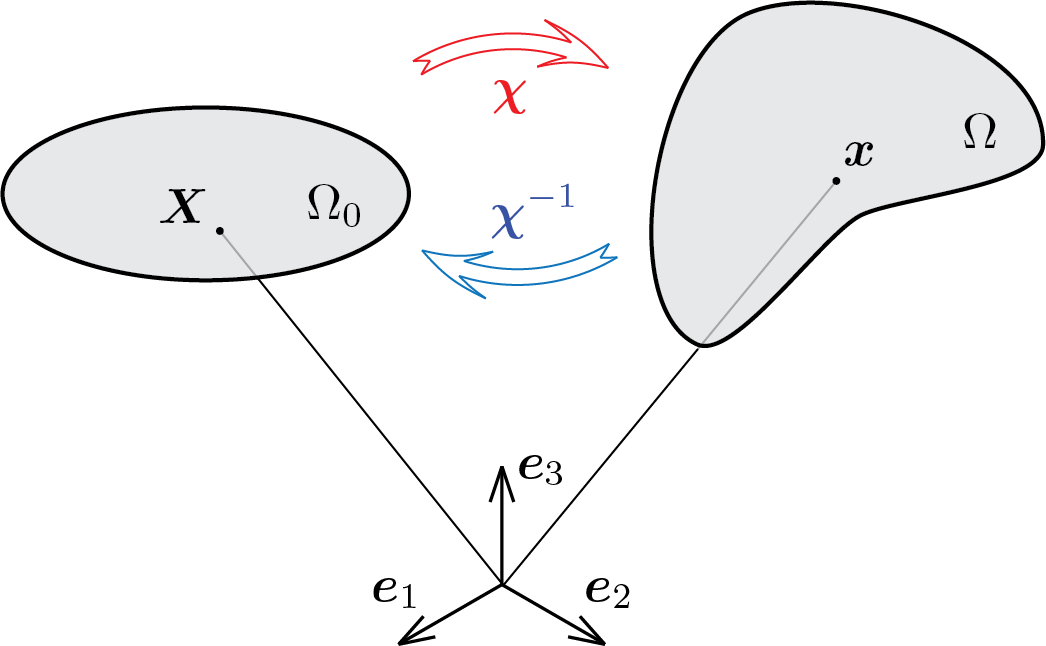
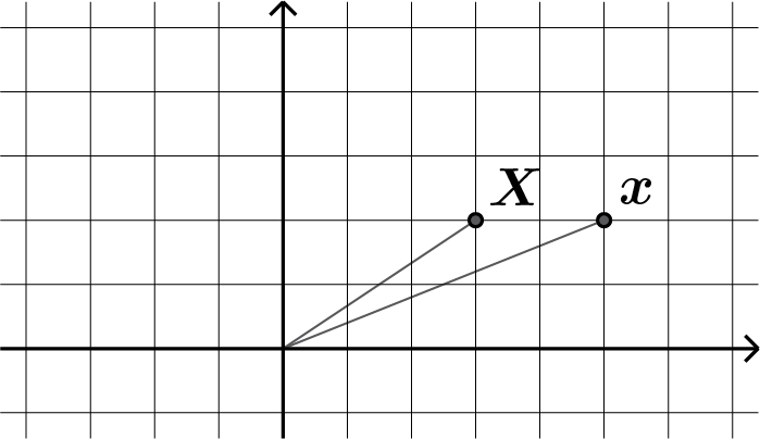
valid \(\forall\vec{X} \in \body_0\text{.}\) \(\vec{\chi}\) is a vector function which, given a position \(\vec{X}\) relative to the reference configuration, provides the new position \(\vec{x}\) relative to the current configuration. The dependence between \(\vec{x}\) and \(\vec{X}\) is sometimes indicated shortly as follows
We assume \(\vec{\chi}\) sufficiently regular to allow derivation up to the desired order.
It is also assumed that the motion \(\vec{\chi} \) is uniquely invertible, i.e. it is possible to write
or
where the symbol \(\vec{\chi}^{-1}\) indicates the inverse motion that associates the current position \(\vec{x}\) with the position \(\vec{X}\) in the reference configuration.
In general the motion \(\vec{\chi}\) of a body will change the position, orientation and shape of the body. A body capable of modifying its shape will therefore be called deformable.
some basic transformations.
Transformation 1 (90 degrees counterclockwise rotation)
![](images/90degreesRotation.png)
Instructions for the definition of a MATLAB® function associated with the assigned transformation and for its use. T1 = @(X) [-X(2); X(1)];
X = [1; 2];
T1(X)
Transformation 2 (horizzontal extension)
![](images/RightExtension.png)
MATLAB® instructions. T2 = @(X) [2*X(1); X(2)];
X = [1; -1];
T2(X)
Transformation 3 (vertical extension)
![](images/UpExtension.png)
MATLAB® instructions T3 = @(X) [X(1); 1.5*X(2)];
v = [4; 10];
T3(v)
Transformation 4 (shear toward right)
![](images/RightShear.png)
MATLAB® instructions T4 = @(X) [X(1)+X(2); X(2)];
u = [10; -1];
T4(u)
The previous examples belong to a very important class of transformations in solid mechanics: linear transformations.
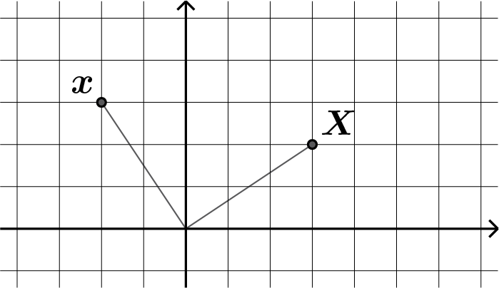
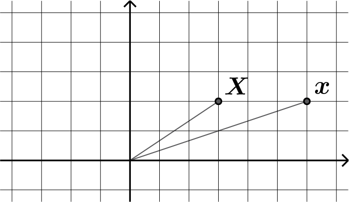
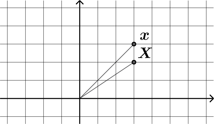
As shown in previous video, in the case in which the transformation \(\vec{\chi}\) is linear its action on the vector \(\vec{X}\) can be transferred through the matrix \(\mat{M_{\chi}}\) defined as follows
where \(\func{\vec{\chi}}{\vec{e}_1}\text{,}\) \(\func{\vec{\chi}}{\vec{e}_2}\) and \(\func{\vec{\chi}}{\vec{e}_3}\) are the vectors obtained by the application of the trasformation \(\vec{\chi}\) to the vectors forming the reference basis. Therefore the transformation of any vector \(\vec{X}\) can be obtained in an equivalent way by applying the matrix \(\mat{M_{\chi}}\text{:}\)
evaluation of the matrix \(\mat{M_{\chi}}\).
In the case of the linear transformations already taken into consideration in the previous examples, it is easy to verify the following results.
Transformation 1
Transformation 2
Transformation 3
Transformation 4
MATLAB® instructions for the creation of the matrices associated with the given transformations. T1 = @(X) [-X(2); X(1)];
T2 = @(X) [2*X(1); X(2)];
T3 = @(X) [X(1); 1.5*X(2)];
T4 = @(X) [X(1)+X(2); X(2)];
M1 = [T1([1; 0]) T1([0; 1])]
M2 = [T2([1; 0]) T2([0; 1])]
M3 = [T3([1; 0]) T3([0; 1])]
M4 = [T4([1; 0]) T4([0; 1])]
Remark 1.2.7.
It is important to underline again that it is possible to identify the matrix \(\mat{M_{\chi}}\) only in the case of linear transformation. Furthermore, the reverse is also true, i.e. the existence of a matrix \(\mat{M_{\chi}}\) usable to represent a transformation implies the linearity of the transformation.