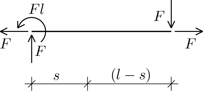
The state of internal stress of one-dimensional solids, or beams, is characterized by evaluating the generalized section forces at each point. In the plane case there are three components: axial force (\(N \)), shear force (\(T \)) and bending moment (\(M \)). In order to come up to a simple definition of these three components, consider the following free body diagram regarding a balanced system of forces.
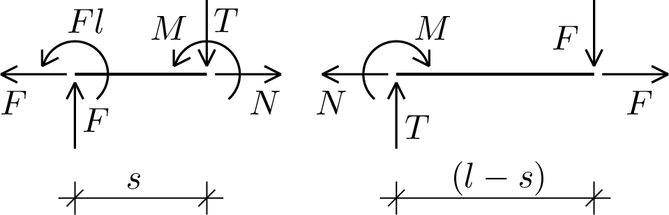
where it is postulated that the two parts exchange, through the separation section, equal and opposite actions. However, these actions must be such as to satisfy the equilibrium equations on each obtained part. In particular, if we consider the part of length \(s \) we obtain the following equations (pole for the rotation equilibrium placed in the abscissa \(s \)):
\begin{align*}
N - F \amp = 0\,,\\
T + F \amp = 0\,,\\
-M - F s + Fl \amp = 0\,.
\end{align*}
System that provides the following solution for the unknown generalized section forces
\begin{align*}
N \amp= F\,,\\
T \amp= -F \,,\\
M \amp= F(l - s)\,.
\end{align*}
The same result would be obtained by applying the equilibrium equations to other part with length \((l-s) \text{.}\)
The separation process carried out can also be understood as the removal of the continuity constraint at point \(s \) and the application of the "constraint reactions" associated with the constraint, of degree 3, removed.
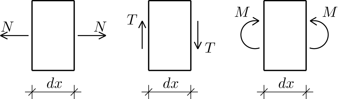
The single sectioning operation must make it possible to obtain two distinct free bodies. If for this purpose one or more sectionings happen to be necessary, the obtained separated parts would lead to the formulation of hyperstatic problems.
By applying the sectioning procedure twice in order to isolate a section of beam of infinitesimal length, it is possible to obtain the following diagram (where the height of the beam has also been made evident) useful for highlighting the convention currently used to define the positive sign for the generalized section forces (for clarity they are shown separately).
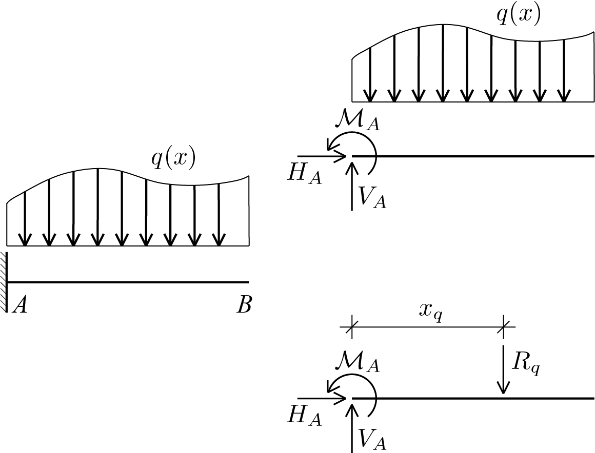
In order to complete the kinds of loads applicable to beam systems and also to make it possible to have a general treatment of the equilibrium diffrential equations presented in the next section, the case of distributed loads is discussed. To this end, consider the following scheme.
The scheme represents a cantilever beam subjected to a variable distributed load \(q (x) \text{.}\) The distributed load is measured as \(\left[\frac{F}{L} \right] \text{.}\) The free body diagram shown at the top right of the figure allows writing the three equilibrium equations (horizontal, vertical and rotation using point \(A \) as pole) providing:
where \(x_q \) represents the centroid of the load with respect to an axis passing through \(A \text{,}\) see the additional free body diagram shown at the bottom right of the figure. Therefore equilibrium equations can be rewritten as follows:
Therefore in systems subjected to distributed loads it is possible to replace the latter with the respective resultants positioned in their centroids. It is observed that this substitution is correct only for the calculation of the constraint reactions and not for the calculation of the generalized cross forces which will be better described later.