Solid Mechanics - applications of the stretched beam model

Section 3.7 applications of the stretched beam model

Subsection 3.7.1 beam simply stretched

Using Equation (3.5.21) calculate the elastic solution for the following scheme.

Due to the absence of a distributed load, the equation to be solved becomes

\begin{equation*} EA\,\frac{d^2u}{dx^2} = 0\,, \end{equation*}

whose general integral is

\begin{equation*} \func{u}{x} = c_0 + c_1 x\,. \end{equation*}

The integration constants can be evaluated by imposing the boundary conditions

\begin{align*} \amp \func{u}{0} = 0\,,\\ \amp \func{N}{l} = EA\, \func{\frac{du}{dx}}{l} = F\,. \end{align*}

From which it can be obtained

\begin{equation*} c_0 = 0\,, \quad c_1 = \frac{F}{EA}\,. \end{equation*}

Then the displacement field takes the following expression

\begin{equation*} \func{u}{x} = \frac{F}{EA} x\,, \end{equation*}

which allows the evaluation of the axial force along the rod and, for example, the movement to the free end

\begin{align*} \amp \func{N}{x} = EA \func{\frac{du}{dx}}{x} = F\,,\\ \amp \func{u}{l} = \frac{F}{EA} l\,, \end{align*}

the latter coincides with the total elongation of the beam, result which can also be obtained as follows

\begin{equation*} \Delta l = \int_l \varepsilon \,dx = \int_l \frac{du}{dx} \,dx = \int_l \frac{F}{EA} \,dx = \frac{F}{EA} \int_l \,dx = \frac{F}{EA} l\,. \end{equation*}

MATLAB® solution.

The general integral can be calculated using the following instructions.

syms u(x) EA;
ode = EA*diff(u,x,2) == 0
dsolve(ode)

Listing 3.7.2.

The solution that also satisfies the assigned boundary conditions is obtained through the following instructions.

syms u(x) EA F l;
Du = diff(u);
ode = EA*diff(u,x,2) == 0;
cond1 = u(0) == 0;
cond2 = EA*Du(l) == F;
conds = [cond1 cond2];
dsolve(ode,conds)

Listing 3.7.3.

Subsection 3.7.2 hyperstatic beam with discontinuity

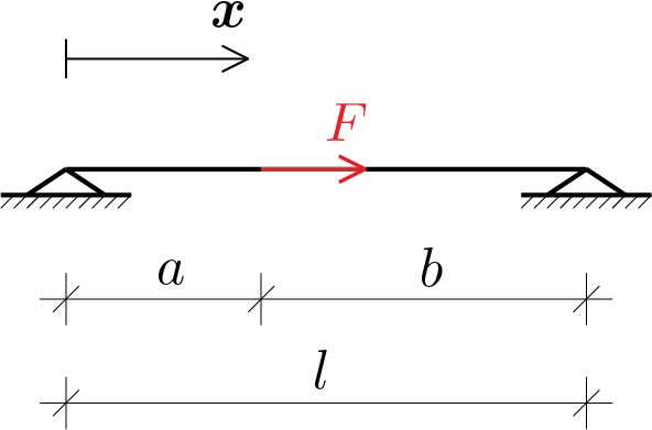
The assigned scheme differs from the scheme considered in the previous section because the elastic solution to be evaluated does not have a single valid expression on the whole domain of the beam. The force applied inside the extension of the beam determines a discontinuity in the solution and therefore the need to study the problem on the two subdomains, \(0 \leq x \leq a \) and \(a \leq x \leq l \text{,}\) highlighted in the figure. We then proceed by evaluating two different elastic solutions but connected by the necessary boundary conditions at the interface.

By applying the equilibrium equation (3.5.21) to the two subdomains the following equations are obtained

\begin{align*} \amp EA\,\frac{d^2u_a}{dx^2} = 0\,,\quad 0 \leq x \leq a\,,\\ \amp EA\,\frac{d^2u_b}{dx^2} = 0\,,\quad a \leq x \leq l\,. \end{align*}

We thus obtain a system of 2 differential equations where the unknowns, \(u_a \) and \(u_b \text{,}\) are uncoupled. Unknowns that still interact in the boundary conditions. In particular, these conditions are expressed by the following equations

\begin{align*} \amp \func{u_a}{0} = 0\,,\\ \amp \func{u_b}{l} = 0\,,\\ \amp \func{u_a}{a} = \func{u_b}{a}\,,\\ \amp EA\, \func{\frac{du_a}{dx}}{a} - EA\, \func{\frac{du_b}{dx}}{a} = F\,, \end{align*}

where the latter equation is given by the static condition

\begin{equation*} \func{N_a}{a} - \func{N_b}{a} = F\,. \end{equation*}

The MATLAB® instructions that can be used for the solution of the system of differential equations are given.

syms ua(x) ub(x) EA F l a;
Dua = diff(ua);
Dub = diff(ub);
ode1 = EA*diff(ua,x,2) == 0;
ode2 = EA*diff(ub,x,2) == 0;
odes = [ode1; ode2];
cond1 = ua(0) == 0;
cond2 = ub(l) == 0;
cond3 = ua(a) == ub(a);
cond4 = EA*Dua(a) - EA*Dub(a) == F;
conds = [cond1 cond2 cond3 cond4];
sols = dsolve(odes,conds);
sols.ua
sols.ub

Listing 3.7.5.

From which we obtain the following solution in terms of the unknown displacements

\begin{align*} u_a \amp= \frac{F}{EA}\frac{l-a}{l}\,x\,,\quad 0 \leq x \leq a\,,\\ u_b \amp= \frac{F}{EA}\frac{l-x}{l}\,a\,,\quad a \leq x \leq l\,. \end{align*}

By calculating the derivative of the obtained solutions, the axial force along the two subdomains takes the following expression

\begin{align*} N_a \amp= EA\, \frac{du_a}{dx} = F\,\frac{l-a}{l}\,,\quad 0 \leq x \leq a\,,\\ N_b \amp= EA\, \frac{du_b}{dx} = -F\,\frac{a}{l}\,,\quad a \leq x \leq l\,. \end{align*}

Subsection 3.7.3 hyperstatic beam subjected to an homogeneous termal increment

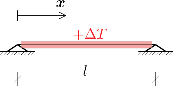
The presence of the increase in temperature determines an elongation of the beam equal to

\begin{equation*} \Delta l_T = \alpha \Delta T \,l\,, \end{equation*}

where \(\alpha \) represents the thermal expansion coefficient of the material. This elongation is however prevented by the presence of the constraints therefore the beam will also be subjected to an axial force calculable by the following equation

\begin{equation*} \Delta l_T + \Delta l_N = \alpha \Delta T \,l + \frac{N}{EA} \,l = 0\,, \end{equation*}

which furnishes

\begin{equation*} N = - EA \,\alpha \Delta T\,, \end{equation*}

solution showing the state of compression determined by the elongation which is not allowed. The solution in terms of displacement is identically zero along its entire beam length.

Subsection 3.7.4 hyperstatic beam subjected to a sinusoidal distributed load

The applied load condition can be expressed as

\begin{equation*} \func{p}{x} = \bar{p}\,\sin\left(\frac{2\pi\,x}{l}\right) \end{equation*}

which, through Equation (3.5.21), gives

\begin{equation*} EA\,\frac{d^2u}{dx^2} + \bar{p}\,\sin\left(\frac{2\pi\,x}{l}\right) = 0 \end{equation*}

to be satisfied in each point of the beam. The boundary conditions are

\begin{align*} \amp \func{u}{0} = 0\,,\\ \amp \func{u}{l} = 0\,. \end{align*}

MATLAB® instructions which can be used to calculate the solution \(\func{u}{x}\) are as follows.

syms u(x) EA p l;
ode = EA*diff(u,x,2) + p*sin(2*pi*x/l) == 0;
cond1 = u(0) == 0;
cond2 = u(l) == 0;
conds = [cond1 cond2];
sol = dsolve(ode,conds)
N = EA*diff(sol,x)

Listing 3.7.8.

The displacement solution is

\begin{equation*} \func{u}{x} = \frac{\bar{p}}{EA} \frac{l^2}{4\pi^2} \sin\left(\frac{2\pi\,x}{l}\right) \end{equation*}

and the axial force is

\begin{equation*} \func{N}{x} = \bar{p} \frac{l}{2\pi} \cos\left(\frac{2\pi\,x}{l}\right)\,. \end{equation*}