Section 3.9 exercises
Subsection 3.9.1
Subsection 3.9.2
In a spot of a thin sheet of aluminum (\(E = 70\,\left[\text{GPa}\right]\text{,}\) \(\nu = 0.3\)) the only non-null strain components are \(\varepsilon_{11} = 0.001\) and \(\varepsilon_{22} = 0.0005\text{.}\)
Analyzing the problem in the plane \((\vec{e}_1,\vec{e}_2)\text{,}\) calculate what follows: principal stresses and principal directions; the stress tensor with respect to a reference system inclined of 30 degrees with respect to the principal directions.
Subsection 3.9.3
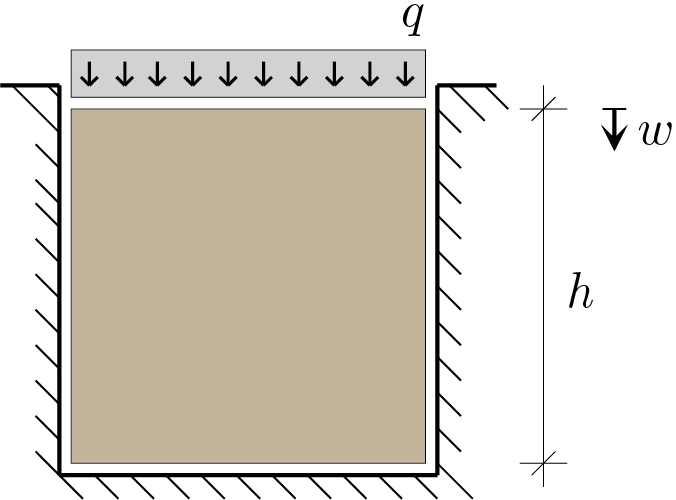
The elastic panel shown above consists of isotropic material with \(E \) and \(\nu \) as generic constituent parameters. The width of the panel coincides exactly with the width of the cavity while in the vertical direction the panel is free to deform without friction phenomena.
Under plane condition, calculate the stress state induced by the application of the load \(q\) and the lowering at the top \(w\text{.}\)
Subsection 3.9.4
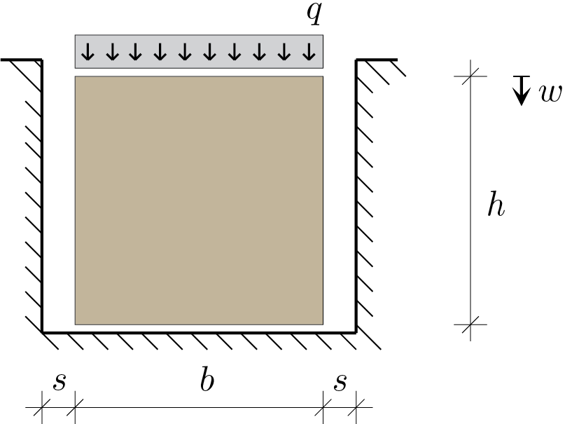
The elastic panel shown above consists of isotropic material with \(E \) and \(\nu \) as generic constituent parameters. The panel is placed in a cavity with perfectly smooth walls.
Under plane condition, calculate the value of the load \(q\) able to match the width of the panel \(b \) with the width, \(b + 2s \text{,}\) of the cavity. Also calculate the lowering at the top \(w\text{.}\)
Subsection 3.9.5
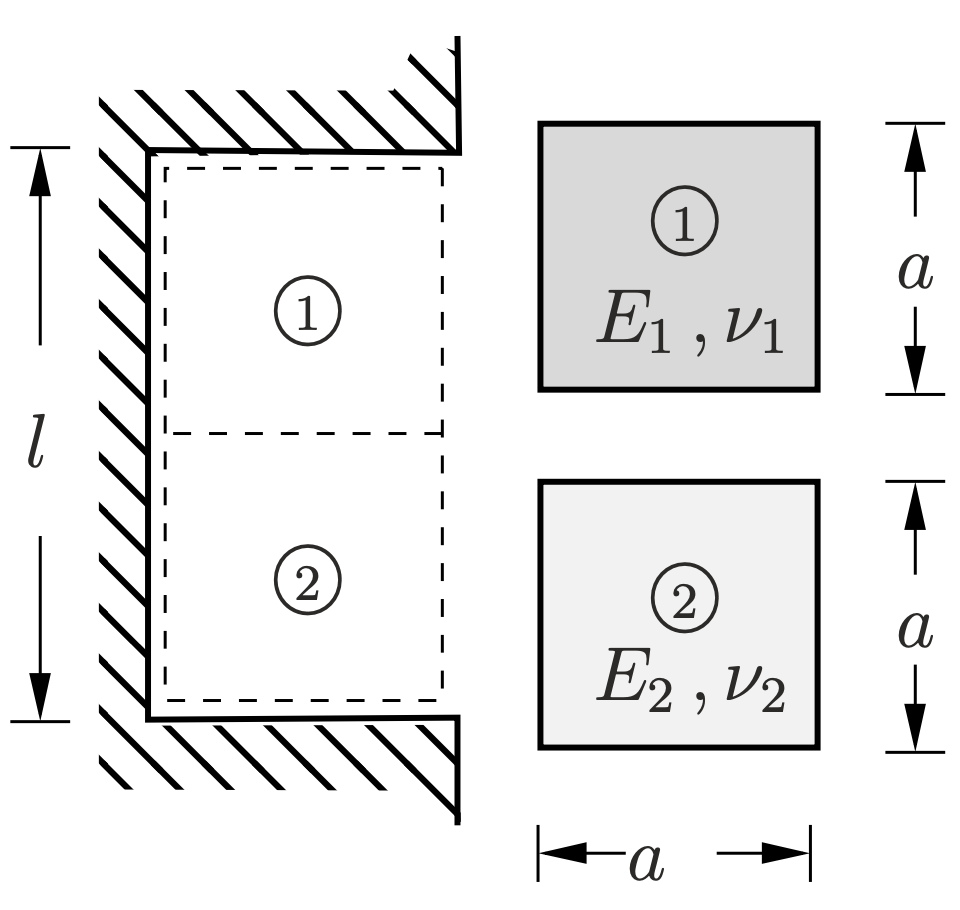
Two square panels of different material are inserted into the cavity with height \(l \) less than \(2a \text{.}\) The elastic problem is solved by assuming no friction phenomena along the cavity walls.
Subsection 3.9.6
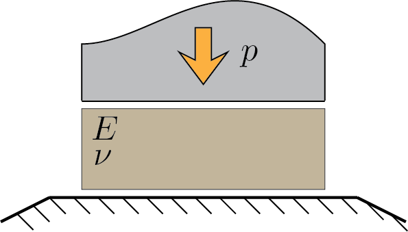
A block of elastic and isotropic material with \(E \) and \(\nu \) generic constituent parameters, is subject to a compression of \(p \) along the axis \(\vec{e}_{3}\text{.}\) Stress and strain components are to be evaluated in the following cases:
-
contrained deformation along directions \(\vec{e}_{1}\) and \(\vec{e}_{2}\text{;}\)
-
contrained deformation along only direction \(\vec{e}_{1}\text{;}\)
-
free deformation along directions \(\vec{e}_{1}\) and \(\vec{e}_{2}\text{.}\)
Subsection 3.9.7
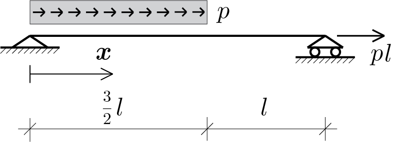
Calculate the elastic solution using the stretched beam model. To this end, assume the Young’s modulus beam equal to the generic value \(E \) and section area equal to \(A \text{.}\)
Once the solution has been obtained, construct a graphical representation of the axial force \(\func{N}{x} \text{.}\)
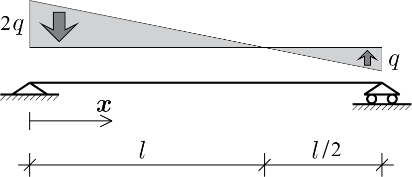
Subsection 3.9.8

Calculate the elastic solution using the stretched beam model. To this end, assume the Young’s modulus beam equal to the generic value \(E \) and section area equal to \(A \text{.}\)
Once the solution has been obtained, construct a graphical representation of the axial force \(\func{N}{x} \text{.}\)
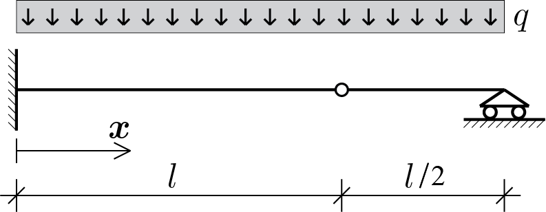
Subsection 3.9.9
Calculate the elastic solution using the bent beam model. To this end, assume the Young’s modulus beam equal to the generic value \(E \) and section moment of inertia equal to \(J \text{.}\)
Once the solution has been obtained, construct a graphical representation of the displacement \(\func{w}{x}\) the bending moment \(\func{M}{x} \text{.}\)
Subsection 3.9.10
Calculate the elastic solution using the bent beam model. To this end, assume the Young’s modulus beam equal to the generic value \(E \) and section moment of inertia equal to \(J \text{.}\)
Once the solution has been obtained, construct a graphical representation of the displacement \(\func{w}{x}\) the bending moment \(\func{M}{x} \text{.}\)
